---
title: "Foundations: Convexity, Gradients, and the Gradient-Based Solver Zoo"
---
This chapter covers the classical foundations every treatment of optimization starts
with — convexity, the gradient, and the family of gradient-based solvers (see e.g.
Brunton [-@brunton2026optimization] or Nocedal & Wright [-@nocedal2006numerical] for
standard textbook treatments) — but every claim below is backed by a from-scratch
implementation in `optimlab` that you can run yourself. Where a textbook proves a
theorem, this chapter shows you the same fact happening to a real solver on a real
landscape.
## What an optimization problem is
::: {.callout-note title="Definition — Optimization problem"}
Given an objective $f: \mathbb{R}^n \to \mathbb{R}$, an **unconstrained optimization
problem** is
$$
\min_{x \in \mathbb{R}^n} f(x).
$$
A point $x^\star$ is a **local minimum** if $f(x^\star) \le f(x)$ for all $x$ in some
neighborhood of $x^\star$, and a **global minimum** if that holds over all of
$\mathbb{R}^n$.
:::
Every solver in `optimlab.optimizers` and every benchmark in
`optimlab.landscapes.testfunctions` speaks the same `Problem` interface — see
`optimlab.core` — specifically so that the code below is not a one-off demo: it's the
exact mechanism the rest of this repo uses.
## Convexity
::: {.callout-note title="Definition — Convex function"}
$f$ is **convex** if for all $x, y \in \mathbb{R}^n$ and $\alpha \in [0, 1]$,
$$
f(\alpha x + (1-\alpha) y) \;\le\; \alpha f(x) + (1-\alpha) f(y).
$$
Geometrically: the line segment connecting any two points on the graph of $f$ never
dips below the graph itself.
:::
::: {.callout-tip title="Theorem — Local minima of convex functions are global"}
If $f$ is convex over a convex feasible set $C$, then every local minimum of $f$ over
$C$ is also a global minimum.
:::
This is *the* reason convex optimization is tractable: a local search algorithm — one
that only ever looks at the gradient right where it's standing — cannot get stuck,
because there's nowhere worse to hide. `optimlab.landscapes` ships both convex
benchmarks (`sphere`, `matyas`) and non-convex ones (`rosenbrock`, `rastrigin`,
`ackley`, `himmelblau`, `beale`, `styblinski_tang`) precisely so you can watch this
guarantee hold on the former and fail on the latter.
## The gradient
::: {.callout-note title="Definition — Gradient"}
For $f: \mathbb{R}^n \to \mathbb{R}$, the gradient is the vector of partial derivatives
$$
\nabla f(x) = \begin{bmatrix} \partial f / \partial x_1 \\ \vdots \\ \partial f / \partial x_n \end{bmatrix},
$$
and it points in the direction of steepest *increase* of $f$ at $x$ — so
$-\nabla f(x)$ is the direction of steepest decrease.
:::
`optimlab.core.Problem` never requires you to hand-derive this: leave `grad=None` and
it's computed exactly via JAX automatic differentiation (falling back to finite
differences if JAX isn't available). Two benchmark functions (`sphere`, `rosenbrock`)
also carry a hand-derived closed form specifically so `tests/test_testfunctions.py` can
check the two agree — worth doing by hand once, not worth doing for every function
after that.
## The solver zoo
Every method below solves the exact same problem — minimize $f$ — by making a
different bet about what information is worth using at each step.
| Solver | Update (schematic) | What it bets on |
|---|---|---|
| Gradient descent | $x_{k+1} = x_k - \alpha \nabla f(x_k)$ | The gradient alone, evaluated at the current point |
| Heavy-ball momentum | $v_{k+1} = \beta v_k - \alpha \nabla f(x_k)$, $x_{k+1} = x_k + v_{k+1}$ | Recent gradient *history* smooths out oscillation |
| Nesterov | as above, gradient evaluated at $x_k + \beta v_k$ | A lookahead gradient corrects momentum before committing |
| Adagrad / RMSProp / Adam | step scaled per-coordinate by (a moving average of) past squared gradients | Different parameters need different effective step sizes |
| Newton | $x_{k+1} = x_k - [\nabla^2 f(x_k)]^{-1} \nabla f(x_k)$ | Curvature (the Hessian), not just slope |
| BFGS / L-BFGS | Newton's step, with the Hessian *approximated* from gradient history alone | Curvature-awareness without ever forming a real Hessian |
The `optimlab.optimizers` docstrings walk through the derivation and trade-offs behind
each row — this table is the map, not the territory.
## Watching it happen: gradient descent zig-zags, Newton doesn't
Standard theory proves gradient descent's convergence rate degrades with a problem's
*condition number* (the ratio of a quadratic's largest to smallest curvature). Rather
than take that on faith, here's the actual zig-zag, on an anisotropic quadratic with
condition number 100:
```{python}
#| label: fig-ill-conditioned
#| fig-cap: "Gradient descent zig-zags across a narrow valley; Newton solves the quadratic model exactly and needs a single step. Contour lines (not just fill color) are what make the zig-zag legible — each line is a level set of equal loss, so tightly packed lines mean the surface is steep there."
import numpy as np

from optimlab.core import Problem
from optimlab.optimizers import bfgs, gradient_descent, newton_method
from optimlab.viz import race_figure


def f(x):
    return 0.5 * (x[0] ** 2 + 100.0 * x[1] ** 2)


def grad(x):
    return np.array([x[0], 100.0 * x[1]])


def hess(x):
    return np.array([[1.0, 0.0], [0.0, 100.0]])


x0 = np.array([10.0, 1.0])
results = {
    "gradient_descent": gradient_descent(
        Problem(f=f, x0=x0.copy(), grad=grad, hess=hess, name="anisotropic_quadratic",
                minimum=np.zeros(2), f_min=0.0, domain=(-11, 11)),
        lr=0.0198, max_iter=1500,  # ~2/(L+mu) for this quadratic — converges in ~900 steps
    ),
    "newton": newton_method(
        Problem(f=f, x0=x0.copy(), grad=grad, hess=hess, name="anisotropic_quadratic",
                minimum=np.zeros(2), f_min=0.0, domain=(-11, 11)),
    ),
}
problem = Problem(f=f, x0=x0.copy(), grad=grad, hess=hess, name="anisotropic_quadratic",
                   minimum=np.zeros(2), f_min=0.0, domain=(-11, 11))

fig = race_figure(problem, results)
fig.show()
```
Gradient descent needs hundreds of small, oscillating steps because a *fixed* step size
has to stay small enough not to overshoot the narrow (high-curvature) direction — and
that same small step size crawls painfully slowly along the wide (low-curvature)
direction. Newton's method uses the Hessian to rescale each direction by its own
curvature and gets there in essentially one step. This is `tests/test_optimizers.py
::test_ill_conditioning_orders_solver_iteration_counts`, made visible.
A top-down contour is a projection — it shows *where* each solver went, not what it
actually descended. The same run, seen as a literal descent down the surface, in 3D:
```{python}
#| label: fig-ill-conditioned-3d
#| fig-cap: "The same race, viewed as an actual descent: gradient descent's zig-zag traces a jagged path down the trough wall; Newton drops almost straight down."
from optimlab.viz import surface_race_figure

surface_race_figure(problem, results).show()
```
Drag to rotate — from directly above this is the same picture as the contour plot;
tilted, gradient descent's path visibly saws back and forth *while* it descends, rather
than looking like a clean diagonal line.
## Watching it happen: four solvers on a genuinely non-convex landscape
Himmelblau's function has four equal-value global minima — a good stress test for
"which basin does each solver fall into," which isn't a question convex optimization
ever has to answer:
```{python}
#| label: fig-himmelblau-race
#| fig-cap: "Four solvers started from the same point on Himmelblau's function — a non-convex landscape with four equal global minima."
from optimlab.landscapes import get
from optimlab.optimizers import ALL_SOLVERS

benchmark = get("himmelblau")
start = [-4.0, 4.0]
race_results = {
    "gradient_descent": ALL_SOLVERS["gradient_descent"](benchmark.problem(x0=start), lr=0.01, max_iter=200),
    "nesterov": ALL_SOLVERS["nesterov"](benchmark.problem(x0=start), lr=0.005, beta=0.8, max_iter=200),
    "newton": ALL_SOLVERS["newton"](benchmark.problem(x0=start)),
    "bfgs": ALL_SOLVERS["bfgs"](benchmark.problem(x0=start)),
}
race_figure(benchmark.problem(x0=start), race_results).show()
```
Himmelblau's landscape is four narrow wells sitting in a much shallower plain — hard to
read off the contour lines alone. In 3D, it's unmistakable:
```{python}
#| label: fig-himmelblau-race-3d
#| fig-cap: "The same four solvers, descending Himmelblau's function in 3D — four sharp wells, one solver in each."
from optimlab.viz import surface_race_figure

surface_race_figure(benchmark.problem(x0=start), race_results).show()
```
And the 2D race, as a convergence curve — note the log-scaled $y$-axis, without which
Newton's and BFGS's curves would be indistinguishable from "instant," and the dotted
extensions: Newton, BFGS, and gradient descent all converge well before Nesterov does,
and stay flat at the optimum rather than the line simply stopping:
```{python}
#| label: fig-himmelblau-convergence
#| fig-cap: "Convergence curves for the same four solvers on Himmelblau's function. Dotted segments mark a solver that already converged, holding its final value out to the longest-running solver in the group."
from optimlab.viz import convergence_figure

convergence_figure(race_results).show()
```
## Try it yourself
Every figure on this page is frozen at whatever code produced it. For a version you can
actually drive — pick a different landscape, drag a learning-rate slider, add or remove
solvers, and watch the plots above re-run live — run the companion
[marimo](https://marimo.io) app locally:
```bash
uv run marimo edit notebooks/marimo/gradient_descent_explorer.py
```
This isn't embeddable on this page: `optimlab` depends on JAX for autodiff, and JAX has
no WebAssembly build, so it can't run inside a browser-only (Pyodide) marimo export the
way a pure-numpy notebook could. What it looks like, running the same Himmelblau race as
above:
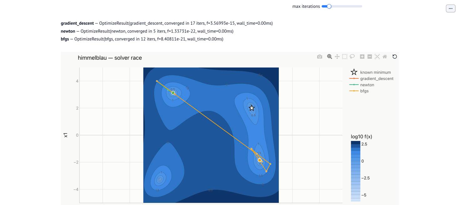
A few things worth trying once it's running: push `gradient_descent`'s learning rate up
on `sphere` until it stops converging (the threshold is exactly $2/L$, where $L$ is
`sphere`'s curvature — its Hessian is $2I$, so $L = 2$); or start from a corner of
`rosenbrock` and compare `gradient_descent` crawling the valley floor against `newton`
or `bfgs` from the same point.
## What's next
This chapter covers the classical, convex-friendly toolkit. The open question this
whole repo exists to chase — *why does any of this still work when $f$ has a billion
parameters and is nowhere near convex* — starts in the high-dimensional non-convexity
module (ROADMAP Phase 6), once linear programming, least squares, and constrained
optimization (Phases 2–4) have built out the rest of the classical toolkit these
solvers eventually get compared against.
