Appendix B — The Testbeds
Every claim in this book is measured against a known truth. This appendix describes the five testbeds in the repository’s src/data_lab/testbeds/: what each computes exactly, how that is checked, and what it cannot show. Each is small enough that every figure runs in under a minute on a laptop, with no network access.
B.1 T2: the long tail, exactly
The setting is Hutter’s toy model (Hutter 2021). Features \(i = 1, 2, \dots\) arrive independently with probabilities \(p_i\), each feature has one fixed label, and the learner memorizes the label of every feature it has seen. It errs exactly on the features it has not seen, so its test error is the \(p\)-mass of the unseen features. With Zipf-distributed features, \(p_i = i^{-(\alpha+1)}/\zeta(\alpha+1)\) for an exponent \(\alpha > 0\).
Uniform sampling. Draw \(n\) training features from \(p\). Hutter’s expected error is
\[ E_n = \sum_{i \ge 1} p_i (1 - p_i)^n \approx c\, n^{-\alpha/(1+\alpha)}, \]
a power law whose exponent is set by the tail (Hutter 2021). The testbed computes the sum exactly, to within a bracket narrower than \(10^{-5}\) of its value. It sums the first \(K\) terms directly. For the rest, \(p_i(1 - n p_i) \le p_i(1-p_i)^n \le p_i\), and both bounds are Hurwitz zeta functions. Checked by tests/test_long_tail.py::test_hutter_exact_sum_matches_monte_carlo (400 seeds) and ::test_learning_curve_slope_approaches_hutter_exponent.
Hutter derives the constant \(c\) for probabilities proportional to \(\alpha\, i^{-(\alpha+1)}\). The same derivation for the normalized \(p_i\) gives \(c = \zeta(\alpha+1)^{-1/(\alpha+1)}\,\Gamma\!\big(\tfrac{\alpha}{1+\alpha}\big)/(\alpha+1)\), which matches the exact sum to 0.1% at \(n = 10^6\) for \(\alpha = 0.5, 1, 2\) (::test_learning_curve_coefficient_for_normalized_zipf).
The oracle coverage selector. Suppose a selector could label the \(n\) most frequent features, never repeating one. Its error is the mass beyond them:
\[ E^{\text{oracle}}_n = \sum_{i > n} p_i, \qquad \frac{(n+1)^{-\alpha}}{\alpha\,\zeta(\alpha+1)} \;\le\; E^{\text{oracle}}_n \;\le\; \frac{n^{-\alpha}}{\alpha\,\zeta(\alpha+1)} . \]
The bounds compare the sum with \(\int x^{-(\alpha+1)}\,dx\) over \([n+1, \infty)\) and \([n, \infty)\), since the summand decreases. The exponent rises from \(\alpha/(1+\alpha)\) to \(\alpha\), but the error is still a power law: removing redundancy steepens it and does not escape it. What remains is the tail mass itself. This selector needs an oracle twice over: it knows which features are already covered, and it knows their frequency order. Checked by ::test_coverage_selection_beats_uniform_at_derived_rate.
It is also optimal: any \(n\) distinct labeled features leave at least this mass, because features \(1, \dots, n\) are the most probable (::test_any_n_labels_cost_at_least_the_tail_mass).
The deduplicated stream. Drop the second oracle: read the uniform stream and label each feature the first time it appears. After \(m\) draws, the labels used and the error are, exactly,
\[ \mathbb{E}[D_m] = \sum_i 1 - (1 - p_i)^m, \qquad E_m = \sum_i p_i (1 - p_i)^m . \]
Writing \(p_i = A\,i^{-s}\) with \(A = 1/\zeta(s)\), \(s = \alpha + 1\), \(\beta = \alpha/(1+\alpha)\), the integral approximation behind Hutter’s eq. 4 gives \(\mathbb{E}[D_m] \approx \Gamma(\beta)\,(Am)^{1/s}\) and \(E_m \approx A^{1/s}\,\Gamma(\beta)\,m^{-\beta}/s\). Eliminating \(m\), at \(n\) labels
\[ E \approx \frac{A\,\Gamma(\beta)^{s}}{s}\,n^{-\alpha} = \beta\,\Gamma(\beta)^{1+\alpha}\cdot\frac{A\,n^{-\alpha}}{\alpha} \approx \beta\,\Gamma(\beta)^{1+\alpha}\,E^{\text{oracle}}_n , \]
the oracle’s exponent at a constant factor (\(\pi/2\) at \(\alpha = 1\)), reached after \(m \approx (n/\Gamma(\beta))^{s}/A\) draws. Both are checked against the exact pair (::test_deduplicated_stream_reaches_the_oracle_exponent_per_label, ::test_deduplicated_stream_pays_n_to_the_one_plus_alpha_draws), and the pair against simulation (::test_deduplicated_stream_exact_curve_matches_simulation).
A selector that knows nothing about \(p\). A realistic selector sees an unlabeled pool of \(M\) draws from \(p\), ranks the distinct features by how often they occur in the pool (ties broken at random), and labels the top \(n\). Whatever the pool, the features it leaves unlabeled include:
- every feature absent from the pool;
- all but \(n\) features, whose mass is at least \(\sum_{i>n} p_i\).
So its error on every pool is at least the larger of the two masses, and in expectation
\[ \mathbb{E}\big[\text{error}\big] \;\ge\; \max\big(E^{\text{oracle}}_n,\; E_M\big), \]
where \(E_M\) is the uniform learning curve at the pool size (checked by ::test_pool_selector_is_bounded_by_unseen_pool_mass). Two consequences follow.
- A pool proportional to the budget, \(M = c\,n\), leaves \(E_M \propto n^{-\alpha/(1+\alpha)}\) against the budget: a constant-factor gain over uniform sampling, and no steeper exponent. Measured at \(\alpha = 1\): slope \(-0.49\) to \(-0.51\) over ten independent sets of seeds (
::test_linear_pool_keeps_the_uniform_exponent). The budget is mostly unspent: such a pool holds about \(\mathbb{E}[D_M] \approx \Gamma(\beta)(AM)^{1/s}\) distinct features, fewer than \(n\) for large \(n\), and the selector labels them all. Against the labels it actually uses, it is the deduplicated stream after \(M\) draws (::test_small_pool_cannot_spend_its_budget). - The oracle’s exponent needs \(E_M \lesssim n^{-\alpha}\), that is, a pool growing like \(M \gtrsim n^{1+\alpha}\). With \(M = n^2\) at \(\alpha = 1\) the selector’s slope was \(-0.99\) to \(-1.01\) over the same ten sets of seeds, at about 1.5 times the oracle’s error (
::test_superlinear_pool_approaches_the_oracle_exponent).
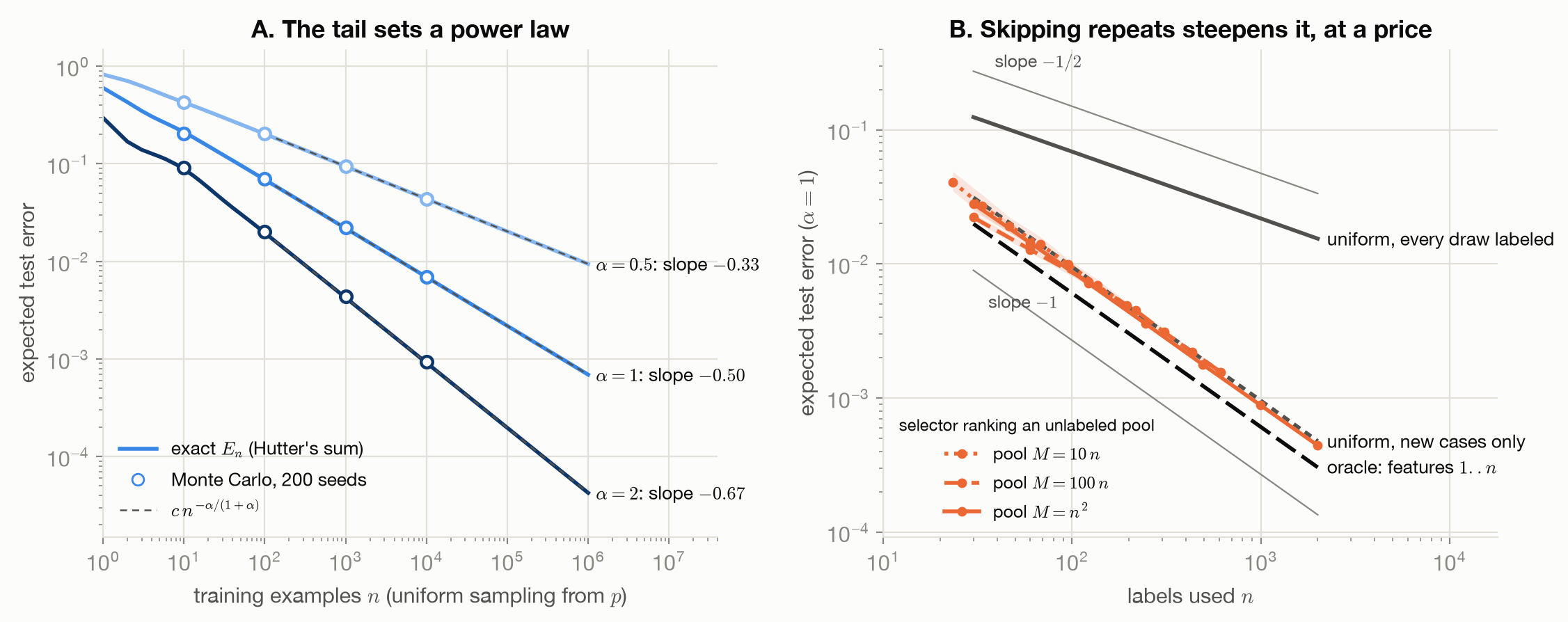
Figure B.1 is the book’s signature figure. It shows the argument of Why Power Laws: The Long Tail. Dohmatob et al. analyze the same model trained on a \(q\) different from \(p\): a cut-off tail, generations of synthetic data, and buying back the missing tail (Dohmatob et al. 2024).
What T2 cannot show. Real inputs are not discrete features with fixed labels, and real learners generalize between inputs rather than memorize them. “Already covered” is trivial here (feature identities are exact); for real data it means near-duplicates or semantic similarity, which have to be estimated. Hutter himself has “no indication that our findings transfer” (Hutter 2021). The testbed shows how a long tail can produce power laws and what selection can and cannot buy in that case, not that real scaling laws arise this way.
B.2 T1: synthetic tabular data
Latent features \(z \sim \mathcal{N}(0, \Sigma)\) with equal correlations, observed as \(x = z\) or, for skewed features, \(x = e^z\). The regression target is log-normal given \(z\): \(\log y = a + b^\top z + \varepsilon\), with \(\varepsilon \sim \mathcal{N}(0, \sigma_\varepsilon(z)^2)\) and optionally heteroscedastic noise. Its conditional mean, median and geometric mean are closed forms, checked against SciPy’s log-normal distribution. The classification target has \(P(y=1 \mid z) = \sigma(u^\top z + u_0)\); the Bayes risk is a one-dimensional integral, checked against the Bayes classifier on 400,000 draws. Covariate shift moves the mean of \(z\) under \(p\), and the density ratio \(w(z) = p(z)/q(z)\) is exact. Missingness masks follow the MCAR, MAR and MNAR definitions (RUBIN 1976), and their dependence structure is checked directly (tests/test_t1_tabular.py).
What T1 cannot show. Real tables have mixed types, unknown dependence and no Bayes risk to compare against.
B.3 T3: the teacher–student perceptron
Sorscher et al.’s theoretical setting (Sorscher et al. 2022):
- Gaussian inputs, \(x \sim \mathcal{N}(0, I)\);
- a teacher drawn uniformly on a sphere, which labels each input by the sign of its projection;
- pruning that keeps the examples with the smallest margin (hard) or the largest (easy);
- a max-margin student.
The test error is exact, \(\phi/\pi\), where \(\phi\) is the angle between student and teacher. A test checks this against 400,000 fresh labeled points. The student is found exactly: finding the shortest \(J\) with every margin at least 1 is a least-distance problem, which reduces to non-negative least squares, solved by an active-set method that terminates. Every solution is certified by its optimality conditions before it is used, and its objective matches a primal reference solver (tests/test_t3_teacher_student.py).
What T3 cannot show. Networks are not perceptrons, and real difficulty scores are noisy estimates of a margin that is known exactly here.
B.4 T4: a Markov text source
The vocabulary’s stationary frequencies are exactly Zipf-like. Transitions mix i.i.d. unigrams with a Metropolis chain that keeps those frequencies, so each token depends on the previous one. The entropy rate is exact: a test checks it by summing over all \(4^5\) sequences of a small instance. It is also the floor on the cross-entropy of any model. Duplicates are injected with exact bookkeeping (tests/test_t4_markov_text.py).
What T4 cannot show. Natural language has long-range structure; a first-order chain has none.
B.5 T5: signals and images
Sums of sinusoids with known frequencies and switch times, analyzed with a short-time Fourier transform, give a known time–frequency structure. Small images come from scikit-learn’s bundled digits, with a synthetic label: whether the left half holds more ink than the right. That label is exactly invariant under an up–down flip and exactly reversed by a left–right flip, so an augmentation is label-preserving or label-changing by construction (tests/test_t5_signals.py).
What T5 cannot show. Real invariances (of a spoken word to pitch, of an object to viewpoint) are approximate and hold only on part of the input space.