11 Learning Curves
“How much data do we need?” is the question this part of the book answers, and the learning curve is the tool for asking it. Plot a model’s expected error against the amount of training data and two features appear: a floor the curve cannot go below, and the rate at which the curve approaches it. This chapter derives both on a task where every point of the curve is exact. It then tests the common practice of estimating the data needed by fitting a curve to a small pilot study and extrapolating.
11.1 The problem
Given a model, a target error and a small dataset, how many examples will reach the target? The honest answer needs three things: what the curve depends on, where its floor is, and how far a curve fitted on few examples can be trusted.
11.2 Assumptions
- A learning curve is an expectation. Following Viering and Loog, the learning curve is the expected risk of the trained model as a function of the training-set size \(n\), averaged over training sets (Viering and Loog 2021, sec. 2). Any single training run is one noisy point.
- The demonstration task is linear and Gaussian. Inputs \(z \sim \mathcal{N}(0, I_d)\); the target is \(a + b^\top z\) plus noise of variance \(\sigma_\varepsilon^2\); the model is least squares. For any fitted coefficients the test risk is exact: \(\sigma_\varepsilon^2 + (\hat a - a)^2 + \lVert \hat b - b \rVert^2\). So every point of the curve is known up to the average over training sets, never up to test-set noise.
- The model and its settings are fixed as \(n\) grows. In practice hyperparameters are retuned for each \(n\), which changes the curve (Viering and Loog 2021, sec. 2.2).
11.3 Derivation or demonstration
The floor. No predictor beats the Bayes risk. For squared error that is the noise variance, \(\sigma_\varepsilon^2\), which is the best possible prediction’s error and does not depend on \(n\). The curve falls toward it and never below (tests/test_learning_curves.py::test_learning_curve_falls_to_the_bayes_floor_scaled_by_noise_and_dimension).
The approach: noise and complexity. For least squares, \(\hat b - b\) is linear in the noise, so on the same inputs and the same noise draws, doubling \(\sigma_\varepsilon\) multiplies the excess risk over the floor by exactly 4 (the test checks this to nine digits). The excess also grows with the number of features \(d\): on this task the measured excess follows \(\sigma_\varepsilon^2 (d + 1)/(n - d - 2)\), within Monte Carlo error, for \(d = 3, 10, 30\) and \(n\) from 100 to 3,000. The data needed for a given excess therefore grows in proportion to both the noise variance and the number of parameters. In this book’s terms, noise sets the floor and the target’s complexity sets how fast the curve gets there.
A learning curve falls toward a floor set by the noise, the Bayes risk, and approaches it at a rate set by how much there is to learn. For least squares on \(d\) features, the excess risk is proportional to the noise variance and grows with \(d\); the training size needed for a fixed excess scales the same way.
Estimating “how much” from a pilot. Viering and Loog review the parametric forms fitted to learning curves. Studies “often find the power law with offset (POW3 in the table) to offer a good fit”, \(E(n) = A\,n^{-B} + C\), where \(C\) is the floor. Some find exponentials or other forms better, and the review reports “strong evidence against the power law in certain settings” (Viering and Loog 2021, sec. 4.1). The procedure tested here is common practice. Take a 200-example pilot. Estimate its error at \(n = 20\) to \(140\) by refitting on subsets and testing on the rest. Fit POW3, and bootstrap the pilot for an interval. The bootstrap must keep copies of a row on one side of each split, or the duplicates leak and the curve looks better than it is (Cleaning).
Over 30 independent pilots:
- The error at \(n = 2{,}000\): the 90% interval contained the true value (1.0055) in 90% of pilots, but its median width was 1.30, larger than the value being estimated (
tests/test_learning_curves.py::test_learning_curve_extrapolation_within_interval). - The data needed for an error 5% above the floor (truth: 230 examples): in 50% of pilots the fitted floor lay above the target, so the answer was “never”.
- With the floor known (fixed at \(\sigma_\varepsilon^2\)), every estimate was finite and every 90% interval contained the truth. The intervals still spanned a median factor of 95.4, and the median point estimate was 130, too low. Over the pilot range the curve falls faster than it does later: the fitted exponent was 1.76 against an asymptotic 1 (
tests/test_learning_curves.py::test_extrapolated_data_requirement_is_biased_and_needs_the_floor).
| Changes | Evaluation only: fits a parametric curve (here POW3, \(A n^{-B} + C\)) to errors measured on subsets of a pilot dataset, and extrapolates |
| Assumption | The fitted form holds beyond the pilot range; the pilot range already shows the asymptotic behavior; the floor \(C\) is identifiable from the pilot |
| What it does to the learned function | None on the model; an estimate, with an interval, of the error at a larger \(n\) or of the \(n\) needed for a target error |
| Which models care | Any model; the estimate is specific to the model and its settings |
| Fit on | The pilot data only, with train/test splits that never put copies of a row on both sides (bootstrap included) |
| Failure modes | The floor is poorly determined, so targets near it are often judged unreachable; the pre-asymptotic curve is steeper than the asymptote, so needed sizes are underestimated; intervals are wide |
| Alternatives | An independent estimate of the noise floor (repeated measurements or labels); collecting a second, larger pilot |
| Checked by | tests/test_learning_curves.py::test_extrapolated_data_requirement_is_biased_and_needs_the_floor |
sklearn.model_selection.learning_curve computes cross-validated scores at several training sizes. Fit the curve to those scores, but treat any extrapolated “data needed” as an order of magnitude, not a number. The single most useful extra measurement is an independent estimate of the noise floor: label a few examples twice, or measure the same item twice.
11.4 What it does to the learned model
Nothing: a learning curve is a measurement, not a technique. What it changes is a decision, whether to collect more data. The demonstration says when that decision is well informed. It is, for gross questions far from the floor (“will 10 times more data help a lot?”). It is not, for fine questions near the floor (“how much for the last 5%?”), because those depend on the floor, which a small pilot cannot see.
11.5 Failure modes
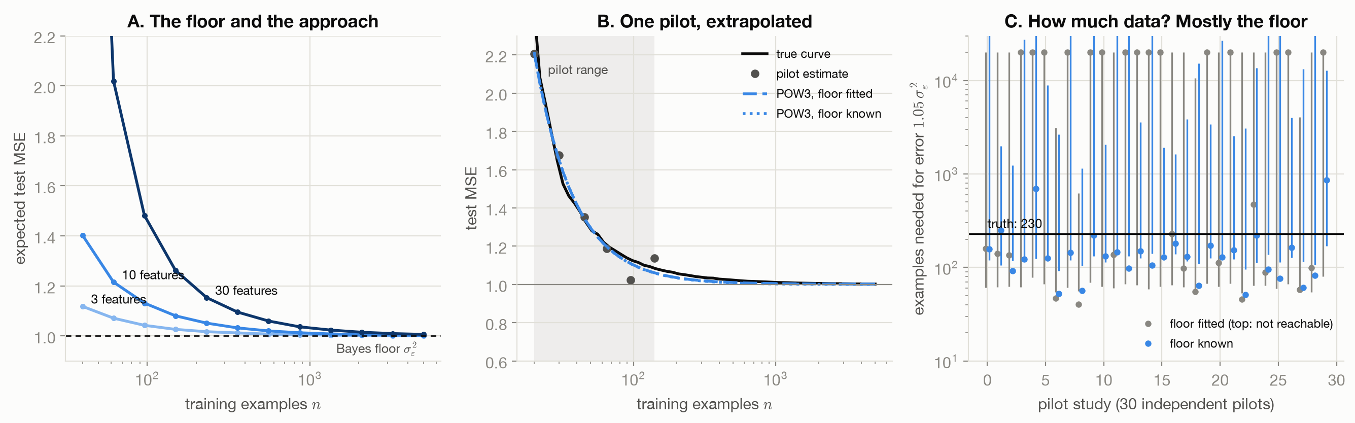
Figure 11.1 shows the curves and the pilot experiment. The failure modes:
- A floor that cannot be seen. Near the floor, the curve’s last few hundredths are invisible in a pilot, and they decide the answer (panel C).
- Pre-asymptotic curves. Early in the curve, error falls faster than it will later. A fit that sees only the early part predicts that the target comes sooner than it does.
- Duplicates in the bootstrap. A bootstrap resample repeats rows. Without grouping the copies, they land on both sides of a pilot’s split, and the intervals for the error at \(n = 2{,}000\) came out less than half as wide: misleadingly confident (
tests/test_learning_curves.py::test_ungrouped_bootstrap_understates_the_interval). - A form that does not fit. POW3 is a common choice, not a law (Viering and Loog 2021, sec. 4.1).
11.6 What the toy cannot show
The task is linear, its noise Gaussian and its model correctly specified, so the curve is smooth and its floor known. Real learning curves can be ill-behaved, “showing worse learning performance with more training data”, for example when the model is misspecified, and they change shape as hyperparameters are retuned (Viering and Loog 2021). Classical generalization bounds give worst-case rates; they are not covered here.
11.7 Connections
- Changing the Shape: the noise level that sets the floor is the same \(\sigma_\varepsilon\) that sets the retransformation gap.
- Scaling Laws: the same curves at the scale of large models, where power laws are reported over many orders of magnitude.
- Why Power Laws: The Long Tail: a mechanism that produces power-law learning curves, and their exponent, exactly.
- Cleaning: Missing Values, Duplicates, Outliers, Leakage: the duplicate leak, which reappears inside the bootstrap.