3 Data Types and Their Structure
A table, a sentence, a photograph and a recording are all arrays of numbers by the time a model sees them. They are not the same kind of array. Each data type has structure the numbers alone do not announce: order, neighborhoods, frequencies, symmetries. A representation either exposes that structure to the model or leaves the model to discover it. And an evaluation either respects it or quietly breaks it. This chapter takes the data types one at a time, then demonstrates both effects: one on the representation lever, one on evaluation.
3.1 The problem
For each data type, three questions decide what preprocessing makes sense:
- What structure is there? Order in time, adjacency in space, a vocabulary with very unequal frequencies, categories without order.
- Which invariances are plausible? A transformation of the input that should not change the target. Plausible is not the same as true: an invariance is an assumption about \(p\), and Augmentation is where assuming it wrongly does harm.
- Which representation exposes the structure? The one under which the target becomes a simple function of the features, for the model at hand.
3.2 Assumptions
- The structure is a property of \(p\), not of the file format. Rows of a table can be ordered in time even when nothing in the table says so.
- The model cannot build every representation itself. A linear model on raw samples cannot compute a spectrum; whether a flexible model learns an equivalent transform depends on its architecture and data, which is outside this book (transformer-atlas covers architectures).
- Evaluation mimics deployment. Validation examples must relate to training examples the way future examples will. If deployment predicts later times, validation must too.
3.3 Derivation or demonstration
Tabular data. Columns are numeric (counts, measurements, money), categorical (no order), ordinal (ordered categories), or dates and times (which carry order, and often cycles). The structure is in the columns’ scales and in which encodings respect them: an ordinal code asserts an order and equal spacing that a categorical column does not have (Encoding and Features). Rows are usually treated as exchangeable. When they are ordered in time they are not, which is the leakage below.
Text. Text is a sequence of tokens from a vocabulary. Word frequencies “approximately [follow] a simple mathematical form known as Zipf’s law”, frequency falling roughly as a power of rank, with “considerable structure” beyond that fit (Piantadosi 2014). Two consequences recur in this book. A few tokens dominate every count, and most of the vocabulary is rare, which is the long tail of Why Power Laws. The Markov text testbed (T4) builds both properties in exactly. Tokenizer internals are out of scope; no sibling book covers them.
Images. An image is a grid of pixel intensities, where neighboring pixels are related. Plausible invariances (a small shift, a change of brightness) are assumptions about the task, not facts about images: a horizontal flip preserves “cat” and destroys “the letter b”. T5 includes a synthetic image label whose invariance under an up–down flip, and reversal under a left–right flip, are exact, for the augmentation experiments.
Audio and the spectrogram. A recording is a waveform sampled at a fixed rate. Frequencies above half the sampling rate cannot be told apart from lower ones. At 8 kHz, the samples of a 5 kHz sine are exactly those of a 3 kHz sine with the sign flipped, since \(\sin(2\pi \cdot 5n/8) = \sin(2\pi n - 2\pi \cdot 3n/8) = -\sin(2\pi \cdot 3n/8)\) (tests/test_data_types.py::test_aliasing_is_exact_above_half_the_sampling_rate). Whatever was above half the rate is folded in before any model sees it.
What distinguishes sounds is usually which frequencies are present, and when. The waveform encodes that only through oscillations whose phase is arbitrary. The spectrogram, the magnitude of a short-time Fourier transform, measures the energy in each frequency band within each short window and discards the phase.
| Changes | Representation (of \(x\)): from samples over time to energy per frequency per time window |
| Assumption | The task depends on which frequencies are present and when, not on their phase; the window is long enough to resolve the frequencies that matter |
| What it does to the learned function | Makes frequency content a feature a linear or local model can use; discards phase, so phase-dependent targets become harder |
| Which models care | Linear and distance-based models, which cannot build the transform themselves; whether a flexible model learns an equivalent front end from raw audio is not tested here |
| Fit on | None: a fixed transform (window length and overlap chosen in advance) |
| Failure modes | Window too short to resolve close frequencies or too long to localize changes in time; aliasing of frequencies above half the sampling rate happens before the transform and cannot be undone |
| Alternatives | Raw waveform with a learned front end; mel or other perceptual frequency scales |
| Checked by | tests/test_data_types.py::test_spectrogram_representation_makes_tone_classes_linearly_separable |
T5 makes the difference concrete. Two classes of noisy tones, 400–600 Hz and 1,200–1,400 Hz, each with a random phase, a quarter second at 8 kHz. Across 400 training and 400 test signals and five seeds, the same regularized logistic regression scores:
- on the raw waveform: a test accuracy of 0.49 to 0.53, chance. With a random phase, the waveform’s distribution is symmetric about zero in both classes, so a linear score cannot separate them and does little better than guessing.
- on the log power spectrum (the time-averaged spectrogram): 1.00 in every seed.
The model did not change; the representation did (tests/test_data_types.py::test_spectrogram_representation_makes_tone_classes_linearly_separable).
Time series. Observations ordered in time are usually autocorrelated: today resembles yesterday. Leakage, in the sense of Kaufman et al., is “the introduction of information about the data mining target, which should not be legitimately available to mine from” (Kaufman et al. 2011). In time, legitimacy has a simple form, which they call a “no-time-machine requirement”: a model may use only what was known before the moment of prediction. Shuffled cross-validation breaks it. Every validation point has training points from just before and just after it.
On T5’s autocorrelated series (a latent AR(1) with coefficient 0.99, plus noise), a 5-nearest-neighbor regressor on the time index was trained on 2,000 steps and evaluated in three ways, over ten seeds:
- shuffled 5-fold cross-validation reported a mean squared error of 1.25;
- time-ordered splits reported 59.5;
- the actual error on the next 300 steps averaged 64.3.
Shuffling understated the error by a factor of at least 14 in every seed (tests/test_data_types.py::test_shuffled_cross_validation_leaks_time).
A representation that makes the target a simple function of the features can turn a task from impossible to trivial for the same model. An evaluation that breaks the data’s ordering measures interpolation instead of prediction. On an autocorrelated series that can understate the error by an order of magnitude or more.
| Changes | Evaluation only: validation examples always come after the training examples in time |
| Assumption | Predictions will be made about later times than the training data; the series is autocorrelated or drifts |
| What it does to the learned function | None on the model; makes the error estimate match the error on the following period on average instead of on interpolated neighbors |
| Which models care | All, most of all those that can interpolate (nearest neighbors, trees, flexible networks) |
| Fit on | Split boundaries set by time stamps |
| Failure modes | Features computed over the whole series (rolling statistics, normalizers) still carry the future into the past; a single future window gives a noisy estimate |
| Alternatives | Blocked cross-validation with gaps; a final held-out future period |
| Checked by | tests/test_data_types.py::test_shuffled_cross_validation_leaks_time |
scipy.signal.stft computes the short-time Fourier transform. Its default window in SciPy 1.18 is 'hann_periodic', so pass window, nperseg and noverlap explicitly. scikit-learn’s TimeSeriesSplit “returns the first k folds as the train set and the (k+1)-th fold as the test set”, and KFold does not shuffle unless shuffle=True (scikit-learn 1.9 docstrings).
Graphs. Nodes connected by edges, where an example’s neighbors carry information about it. Graph representations are covered in modern-ai-systems-and-methods; the leakage lesson transfers, since a node’s neighbors in a validation set may sit in the training set.
3.4 What it does to the learned model
A representation sets which functions are simple. The spectrogram did not add information to the tones; it moved the information into a form a linear model can read. The same move recurs in Changing the Shape and Encoding and Features.
An evaluation split changes nothing about the model and everything about what we believe of it. The nearest-neighbor model was the same in all three columns of the comparison; only the estimate of its error moved.
3.5 Failure modes
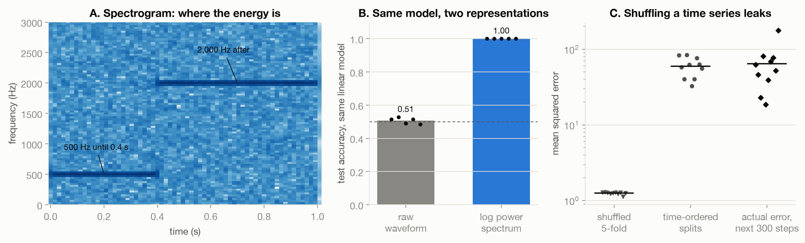
Figure 3.1 shows the three effects. Failures that follow from them:
- A spectrogram with the wrong window. A short window cannot resolve close frequencies; a long one smears changes in time.
- Leakage that survives a time-ordered split. Features computed over the whole series (a normalizer, a rolling average centered on each point) carry the future into the past. This is the leaking-features case of Kaufman et al.
- A noisy future window. In the demonstration the time-ordered estimate matched the future error on average. Any one 300-step future window, though, varied by nearly a factor of ten across seeds (18.6 to 176.6).
3.6 What the toy cannot show
The tones differ in one obvious feature and the series has one source of dependence. Real audio needs perceptual frequency scales and longer context. Real time series mix trends, seasonality and changes in regime. Both demonstrations show the direction and the mechanism of an effect, not its size on real data.
3.7 Connections
- Labels: what counts as one example (a clip, a window, a user) also decides what counts as a mislabeled one.
- Cleaning: Missing Values, Duplicates, Outliers, Leakage: leakage through fitted preprocessing, the non-temporal relative of the shuffled split.
- Augmentation: the plausible invariances listed here, turned into training data, and what happens when one is wrong.
- Why Power Laws: The Long Tail: text’s Zipf-like frequencies are the long tail that makes returns on data diminish.