14 Choosing Data
If returns on data diminish because most examples repeat what is already learned (Why Power Laws: The Long Tail), then choosing which examples to keep, label or train on should help. A whole literature does this: deduplication, pruning by difficulty, active learning, loss-based selection, domain mixtures and large-scale filtering. Its reverse is training on data a model generated, which chooses badly by construction. Every one of these methods pulls the same lever, the sampling distribution \(q\), and every one works only under a condition. This chapter measures four of the conditions and states the rest from their sources.
14.1 The problem
Given more candidate data than can be used (or labeled, or trained on), which examples should the model see? When does choosing beat drawing at random, and when does it do harm?
14.2 Assumptions
- Selection changes \(q\), deliberately. The chosen examples are not a sample of \(p\), so anything estimated from them, including the model’s own validation error, is biased unless corrected (The Data-Generating Process).
- Each demonstration uses the testbed that makes its condition exact: T3 for pruning (example difficulty known), T4 for deduplication (duplicates and entropy rate known), T1 for active learning (Bayes rule known), and T2 for synthetic data (the tail known).
- Large-scale methods are stated, not reproduced. Their results are labeled as reported, with dates.
14.3 Derivation or demonstration
Pruning by difficulty (replicated finding with conditions; the crossover is from one theory paper, 2022). Sorscher et al. analyze pruning in the teacher–student perceptron, the setting of T3. Their result: “with abundant (scarce) initial data, one should retain only hard (easy) examples” (Sorscher et al. 2022, sec. 1), and with an increasing pruning fraction error can fall faster than a power law, given “a high-quality data pruning metric” [abstract]. On T3 with 100 dimensions, keeping half the examples by their true margin:
- scarce data (\(P/N = 1\)): keeping the easiest half gave test error 0.255, the hardest half 0.402, a random half 0.327; hard beat easy in 0 of 20 seeds;
- abundant data (\(P/N = 16\)): hardest half 0.0295, easiest 0.0380, random 0.0586; hard beat easy in 18 of 20 seeds (
tests/test_pruning.py::test_pruning_crossover_hard_when_abundant_easy_when_scarce).
In between, at \(P/N = 4\), hard won in 10 of 20. Real difficulty scores estimate the margin. Paul et al.’s EL2N (the norm of a model’s error vector early in training) and GraNd (the expected gradient norm) (Paul et al. 2021), Toneva et al.’s forgetting events (Toneva et al. 2018), and scores from small proxy models (Coleman et al. 2019) all do so. Ayed and Hayou report that random pruning “outperforms most existing data pruning methods in the high compression regime” and prove limits for score-based pruning (Ayed and Hayou 2023, abstract).
| Changes | Sampling distribution \(q\): keeps a fraction of the training set ranked by a difficulty score (margin, EL2N, GraNd, forgetting events) |
| Assumption | The score ranks examples as the true margin would; the right end to keep depends on how much data there is |
| What it does to the learned function | Keeping hard examples sharpens the boundary when data is abundant; keeping easy ones gives coarse information first when it is scarce |
| Which models care | Demonstrated for a max-margin perceptron; reported for image networks |
| Fit on | Scores from a probe model trained on the training data (a few epochs, or a different architecture) |
| Failure modes | Keeping hard examples with scarce data; noisy scores at high pruning rates, where random pruning can win (Ayed and Hayou); hard examples that are mislabeled |
| Alternatives | Random subsampling; self-supervised scores; reweighting instead of discarding |
| Checked by | tests/test_pruning.py::test_pruning_crossover_hard_when_abundant_easy_when_scarce |
Deduplication (replicated finding). Lee et al. found near-duplicates and long repeated substrings in standard language-model corpora: “over 1% of the unprompted output” of models trained on them was copied verbatim, and one 61-word sentence was repeated “over 60,000 times”. Deduplicated models emitted memorized text “ten times less frequently” and reduced train–test overlap (Lee et al. 2021, abstract). On T4, 50 of 400 documents were each copied five extra times, and a trigram model that can memorize documents was trained on an 80/20 split:
- with duplicates across the split (45% of test documents also in training): the measured test cross-entropy was 0.45 nats lower than on fresh text, between 0.31 and 0.56 across 20 seeds;
- deduplicated before splitting: within 0.11 nats of the fresh-text value (
tests/test_dedup.py::test_deduplication_reduces_overlap_optimism).
On a long tail, deduplication also has a second role, measured in Why Power Laws: it stops labels being spent on covered cases.
| Changes | Sampling distribution \(q\) and weights: removes repeated examples, which also removes their extra weight in the loss |
| Assumption | Repeats are artifacts of collection, not part of \(p\); what counts as a repeat (exact or near) can be defined |
| What it does to the learned function | Less memorization of repeated content; evaluation that measures generalization rather than recall; on a long tail, labels are not spent on covered cases |
| Which models care | Most visible for models that memorize (large language models, nearest neighbors) |
| Fit on | The whole corpus, before any split |
| Failure modes | Near-duplicates missed by exact matching; deduplicating genuine frequency information away; deduplicating after splitting |
| Alternatives | Down-weighting repeats; group-aware splits |
| Checked by | tests/test_dedup.py::test_deduplication_reduces_overlap_optimism |
Active learning. Uncertainty sampling “queries the instance whose posterior probability of being positive is nearest 0.5” (Settles 2009, sec. 3.1). On T1, starting from 10 random labels and adding 90 one at a time, it reached a rule closer to the Bayes rule than random labeling when the classes were nearly separable: at 100 labels it had 0.57 times random’s disagreement (Bayes risk 0.08). The gain vanished as label noise grew: the ratio was 0.97 at a Bayes risk of 0.25, and 1.07 at higher noise (60 seeds; tests/test_active_learning.py::test_uncertainty_sampling_gains_shrink_with_label_noise). Near a noisy boundary, the most uncertain examples are mostly noise. A 20-seed pilot suggested that uncertainty sampling was worse than random there; with 60 seeds the difference was within noise.
| Changes | Sampling distribution \(q\): the next example to label is the pool example the current model is least sure about |
| Assumption | Uncertainty reflects what the model has not learned, not irreducible label noise; the pool represents \(p\) |
| What it does to the learned function | Labels concentrate near the current boundary, which helps when classes are nearly separable |
| Which models care | Probabilistic classifiers that are refit as labels arrive |
| Fit on | The labeled set so far and an unlabeled pool |
| Failure modes | Noisy labels: uncertainty points at noise, and the gain vanishes; the labeled set is no longer a sample of \(p\) (biased estimates); querying outliers |
| Alternatives | Random labeling; diversity- or density-weighted selection; RHO-LOSS-style criteria |
| Checked by | tests/test_active_learning.py::test_uncertainty_sampling_gains_shrink_with_label_noise |
Selection by learnability (single study, 2022). Mindermann et al. select, within each batch, the points whose training loss most exceeds an “irreducible holdout loss”: the loss of a small model trained on holdout data. This avoids points that are already learned and points that are noisy, which plain high-loss selection picks. They report reaching target accuracy in 18 times fewer steps on a web-scraped, noisily labeled benchmark (Mindermann et al. 2022).
| Changes | Sampling distribution \(q\): within each batch, trains on the points whose training loss most exceeds the loss of a small model trained on holdout data |
| Assumption | Holdout data from \(p\) is available; a small model’s loss estimates what is irreducible (noise) for each point |
| What it does to the learned function | Skips points that are already learned and points that are noisy or unlearnable, which plain high-loss selection would pick |
| Which models care | Reported for neural networks trained by SGD |
| Fit on | A holdout set, through the irreducible-loss model |
| Failure modes | A poor irreducible-loss model misjudges noise; holdout data that is not from \(p\) |
| Alternatives | Uniform sampling; uncertainty or high-loss selection |
| Checked by | Not tested here; stated from (Mindermann et al. 2022) |
Mixtures and filtering at scale (reported, 2023–2024). DoReMi sets the proportions of training domains with a small proxy model trained by group distributionally robust optimization. It reports reaching a baseline’s downstream accuracy “with 2.6x fewer training steps” (Xie et al. 2023, abstract). DataComp makes dataset filtering itself the benchmark, with a pool of 12.8 billion image–text pairs (Gadre et al. 2023). FineWeb documents a 15-trillion-token web dataset and ablates its curation choices (Penedo et al. 2024). Goyal et al. show that the best filter depends on the training budget: limited high-quality data “rapidly loses its utility when repeated”, so data curation “cannot be agnostic of the total compute” (Goyal et al. 2024, abstract).
| Changes | Sampling distribution \(q\): the proportion of training data drawn from each domain |
| Assumption | Weights found by a small proxy model transfer to a larger model |
| What it does to the learned function | Reported to reach a baseline’s downstream accuracy in fewer steps |
| Which models care | Reported for language models |
| Fit on | A small proxy model trained with group distributionally robust optimization over domains |
| Failure modes | Weights that do not transfer to the larger model or to the target task |
| Alternatives | Default or hand-tuned proportions; mixture scaling laws |
| Checked by | Not tested here; stated from (Xie et al. 2023) |
| Changes | Sampling distribution \(q\): keeps the documents a quality filter scores highly |
| Assumption | The filter’s notion of quality predicts usefulness for the target; enough data remains for the compute available |
| What it does to the learned function | Reported to give better models for the same training budget when the filter is good; benchmarks such as DataComp compare filters directly |
| Which models care | Large models trained on web data |
| Fit on | Heuristics or classifiers, sometimes trained on reference data |
| Failure modes | Filtering away rare but needed content (the tail); filtering choices that are right for one compute budget and wrong for another (Goyal et al.) |
| Alternatives | Deduplication only; reweighting by quality instead of discarding |
| Checked by | Not tested here; stated from (Goyal et al. 2024) |
Training on generated data (replicated finding, with a contested scope). Shumailov et al. report that training on model-generated data loses the tails of the original distribution (Shumailov et al. 2023, 2024; an author correction was published in 2025, Shumailov et al. 2025, whose content could not be accessed). Dohmatob et al. derive the consequence on Hutter’s model. A generator fit to \(t_0\) samples cuts the tail, and a learner trained on its output plateaus (Dohmatob et al. 2024, Thm 2.1 and Cor. 2.2). Gerstgrasser et al. find that collapse follows when synthetic data replaces real data, and is avoided when the two accumulate (Gerstgrasser et al. 2024). On T2 (\(\alpha = 1\), \(t_0 = 10{,}000\) draws per generation, 20 seeds), the mass outside the generator’s support was 0.0069 in the first generation, equal to Hutter’s expected error at \(t_0\) (0.0069). Replacing the data each generation, it grew to 0.0167 by the tenth. Accumulating, it never grew (tests/test_collapse.py::test_refitting_on_own_samples_loses_tail). A learner trained on generated data can never get below that lost mass, however much it sees (::test_training_on_generated_data_plateaus_at_the_lost_mass).
| Changes | Sampling distribution \(q\): training examples are drawn from a fitted model instead of from \(p\) |
| Assumption | The generator’s distribution covers \(p\), including its tail |
| What it does to the learned function | A generator fit to finite data misses the unseen tail; a learner trained on its output plateaus at that missing mass |
| Which models care | Every model trained on generated data |
| Fit on | The generator’s own training data |
| Failure modes | Replacing real data generation after generation loses more of the tail each time; accumulating real and synthetic data does not |
| Alternatives | Keeping and reusing the real data; mixing a share of fresh real data |
| Checked by | tests/test_collapse.py::test_refitting_on_own_samples_loses_tail |
Choosing data changes \(q\), and each method helps only when its condition holds. Keeping hard examples needs abundant data. Uncertainty sampling needs labels whose noise is small near the boundary. A test set needs to be deduplicated against training. Loss-based selection needs a way to tell unlearned from unlearnable. Training on generated data needs the real data kept, because a generator fit to finite data has already lost the tail.
Deduplicate before splitting, exactly and then approximately. Prefer weighting to discarding when unsure. Before trusting a selection method, compare it with random selection at the same budget, on your data, with several seeds. Keep the real data you have: if synthetic data is added, add it, never substitute it.
14.4 What it does to the learned model
Selection changes what the model sees, so it changes what the model is good at. Pruning toward hard examples spends the budget near the boundary; keeping easy ones teaches the bulk first. Active learning, by design, makes the labeled set unrepresentative of \(p\). Training on generated data teaches the generator’s distribution, tail missing. In every case the model’s own validation numbers, if computed on the selected data, describe \(q\), not \(p\).
14.5 Failure modes
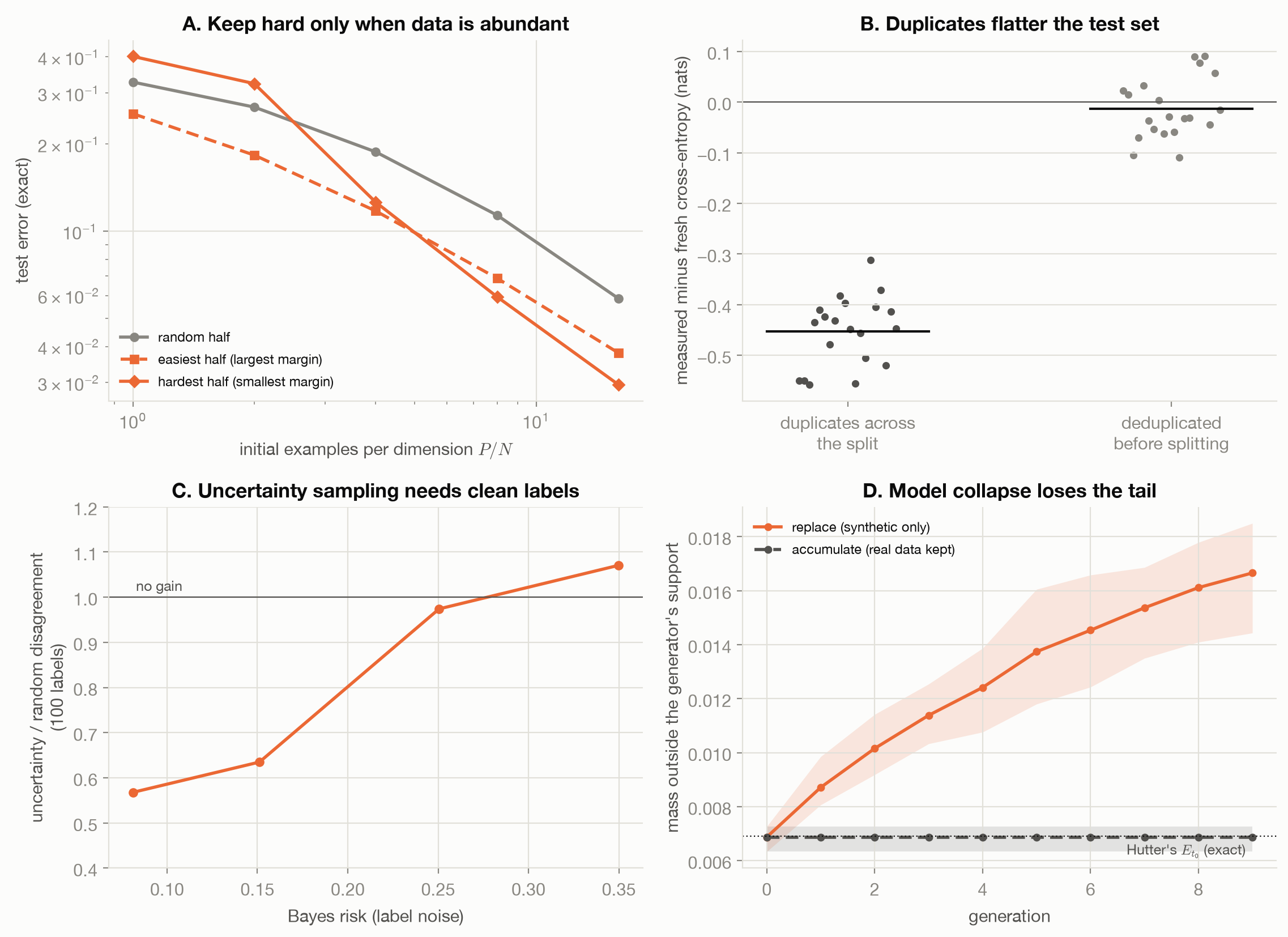
Figure 14.1 shows the four conditions failing:
- Pruning the wrong end for the amount of data (panel A).
- Evaluating on duplicates (panel B).
- Querying noise (panel C).
- Replacing real data with generated data (panel D).
- Selection tuned at one scale used at another. A filter or mixture chosen for one compute budget can be wrong for another (Goyal et al. 2024).
14.6 What the toy cannot show
Each testbed isolates one condition. Real selection methods face several at once, use estimated scores instead of true margins and posteriors, and run at scales where comparing with random selection is itself expensive. The large-scale results above are reported by their authors, on their data, as of their publication; they are not reproduced here.
14.7 Connections
- Why Power Laws: The Long Tail: what coverage-driven selection can and cannot buy, exactly, on the long tail.
- Sampling and Weighting: when a selection rule is known, weights can undo its bias, at a cost in variance.
- Cleaning: Missing Values, Duplicates, Outliers, Leakage: the same duplicate leak on tabular data.
- rl-for-llms, Imitating a Better Distribution: training on a model’s own filtered samples, where the generator is the model being trained.