5 Affine Scaling
Most preprocessing pipelines scale features before anything else, usually with whichever scaler the tutorial used. The four common scalers look like four choices. They are one operation with four choices of constants, and that operation leaves most of what matters about a feature untouched. What it changes is the yardstick: the units in which distances are measured, penalties are charged and gradients are taken. This chapter separates what scaling cannot do from what it does, and finds the one case where the choice of scaler decides the outcome.
5.1 The problem
A feature measured in meters and another in millimeters differ by a factor of 1,000 that means nothing about the world. Some models do not notice; others are dominated by the larger number. Which are which, and what exactly does a scaler change?
5.2 Assumptions
- Each feature is transformed separately, by \(x_j \mapsto (x_j - a_j)/b_j\) with \(b_j > 0\) fit on training data. Transforms that mix features (whitening, PCA) are different operations.
- Distances and penalties are computed on the transformed features. A model that rescales internally, or a tree that only compares values within a feature, is unaffected by construction.
- “Outlier” means a gross error or a rare extreme value, a small share of the data. If a quarter of a feature is extreme, it is the distribution, not an outlier.
5.3 Derivation or demonstration
The four scalers in scikit-learn 1.9 all have the form \((x_j - a_j)/b_j\):
| Scaler | Center \(a_j\) | Scale \(b_j\) |
|---|---|---|
StandardScaler |
mean | standard deviation (biased, ddof=0) |
MinMaxScaler |
minimum | maximum minus minimum |
MaxAbsScaler |
0 | maximum absolute value |
RobustScaler |
median | interquartile range (25th to 75th percentile) |
(Read from the scikit-learn 1.9 docstrings.) An increasing affine map changes a feature’s location and spread and nothing else. Every standardized moment, \(\mathbb{E}\big[(x - \mathbb{E}x)^k\big] / \mathrm{Var}(x)^{k/2}\), is unchanged, because the shift cancels in \(x - \mathbb{E}x\) and the scale cancels between numerator and denominator.
Standard, min-max, max-abs and robust scaling leave every feature’s skewness and kurtosis exactly as they were. A skewed feature stays skewed, and a heavy tail stays heavy. Changing the shape takes a nonlinear transform (Changing the Shape).
On T1’s log-normal features, all four scalers reproduce the input’s skewness and kurtosis to nine significant digits, and each output column is an exact increasing line of its input (tests/test_scaling.py::test_affine_scalers_preserve_skewness_and_kurtosis).
Which models care. Three kinds of model see units; one does not.
- Distance-based models. A nearest-neighbor classifier’s distance sums squared differences across features, so a feature on a large scale dominates. Constructed case: a query at \((0, 0)\), neighbor A at \((1, 0)\) of class 0, neighbor B at \((0, 10)\) of class 1. The nearest neighbor is A. Divide the second feature by 100 and B is at distance 0.1: the prediction flips. On T1, putting one of three informative features on a scale 100 times larger lowered a 15-nearest-neighbor classifier’s test accuracy from 0.729 to 0.603 (20 seeds); at 300 times it fell to 0.563 (Figure 5.1). Standardizing restored 0.729 at every scale (
tests/test_invariance.py::test_knn_prediction_flips_under_feature_rescaling). - Penalized models. A penalty such as a constant times \(\sum_j \theta_j^2\) charges every coefficient the same price, but a feature in millimeters needs a coefficient 1,000 times smaller than the same feature in meters. Scaling decides which features the penalty shrinks most.
- Gradient-trained models. For least squares, the Hessian is \(D^\top D/n\), where \(D\) is the design matrix with a column of ones. With T1’s features on scales 1, 100 and 0.01, and the first offset by 50, its condition number was \(1.2 \times 10^8\); standardized, it was 2.35. How such a condition number slows gradient descent, through a zig-zag across a narrow valley, is shown in optimization-lab (
tests/test_scaling.py::test_feature_scaling_changes_least_squares_conditioning). - Trees. A decision tree splits one feature at a time on thresholds, and an increasing transform keeps every ordering, so it keeps every candidate split. On T1, under affine, log, square-root and cube transforms, the tree’s predictions on its training points were identical in every one of ten seeds. There is a fine print, found by testing rather than assumed. scikit-learn places each threshold halfway between the two adjacent values in the node (
tests/test_invariance.py::test_tree_thresholds_are_midpoints_within_each_node), and a nonlinear map does not keep midpoints. A new point falling in such a gap can switch sides. On 20,000 new points per seed, an affine transform changed no prediction, and the nonlinear ones changed at most 0.16% (tests/test_invariance.py::test_tree_predictions_invariant_to_monotone_feature_transform).
| Changes | Representation (of \(x\)): each feature is shifted and divided by a positive constant |
| Assumption | The model’s behavior depends on the features’ units; a feature’s typical spread is a fair yardstick for its importance |
| What it does to the learned function | None on the shape of any feature (skewness and kurtosis unchanged); equalizes the units that distances and penalties compare; improves the conditioning of a least-squares fit |
| Which models care | Distance-based models (nearest neighbors, kernels, clustering), penalized models, gradient-trained models; not trees, and not unpenalized linear models’ predictions |
| Fit on | Training data only: mean and standard deviation, or minimum and maximum, or maximum absolute value |
| Failure modes | Outliers set the scale (standard and min-max); a feature that should matter more is made to matter equally; test values outside the training range (min-max) |
| Alternatives | Robust scaling; a shape-changing transform when the problem is skew, not units |
| Checked by | tests/test_scaling.py::test_affine_scalers_preserve_skewness_and_kurtosis |
Outliers. The mean, the standard deviation, the minimum and the maximum all move with a single extreme value. With 1% of a standard normal sample replaced by values near 100, the standard deviation is inflated about tenfold. After StandardScaler, the remaining 99% of the data had a spread of 0.10: squeezed into a narrow band that every distance and penalty now treats as nearly constant. The median and quartiles barely move. After RobustScaler, the inliers’ spread was 0.74, the same as without outliers, where \(0.74 = 1/1.349\) and 1.349 is the interquartile range of a standard normal (tests/test_scaling.py::test_robust_scaler_keeps_inlier_spread_under_outliers).
| Changes | Representation (of \(x\)): each feature is centered at its median and divided by its interquartile range |
| Assumption | Outliers are a small share of each feature (fewer than a quarter on each side) |
| What it does to the learned function | Same as affine scaling for the bulk of the data, with a scale that outliers cannot inflate; the outliers themselves stay extreme |
| Which models care | The same models as affine scaling |
| Fit on | Training data only: median and quartiles |
| Failure modes | Outliers are left in place at large values; features with an interquartile range of zero (mostly constant) |
| Alternatives | Removing errors before scaling; clipping; a shape-changing transform; a robust loss (loss-functions-lab) |
| Checked by | tests/test_scaling.py::test_robust_scaler_keeps_inlier_spread_under_outliers |
Fit the scaler inside a Pipeline so it sees training folds only (Cleaning). RobustScaler’s quantile_range defaults to (25.0, 75.0). MinMaxScaler maps the training range to feature_range=(0, 1); test values outside the training range land outside it unless clip=True.
5.4 What it does to the learned model
For an unpenalized linear model with an intercept, scaling changes nothing about the predictions: the coefficients absorb the constants. For a tree, it changes nothing on the training data and almost nothing elsewhere. For everything that measures distances, charges penalties or follows gradients, it changes which features count and how fast training converges. The data’s shape, the thing a model is actually fit to, is untouched.
5.5 Failure modes
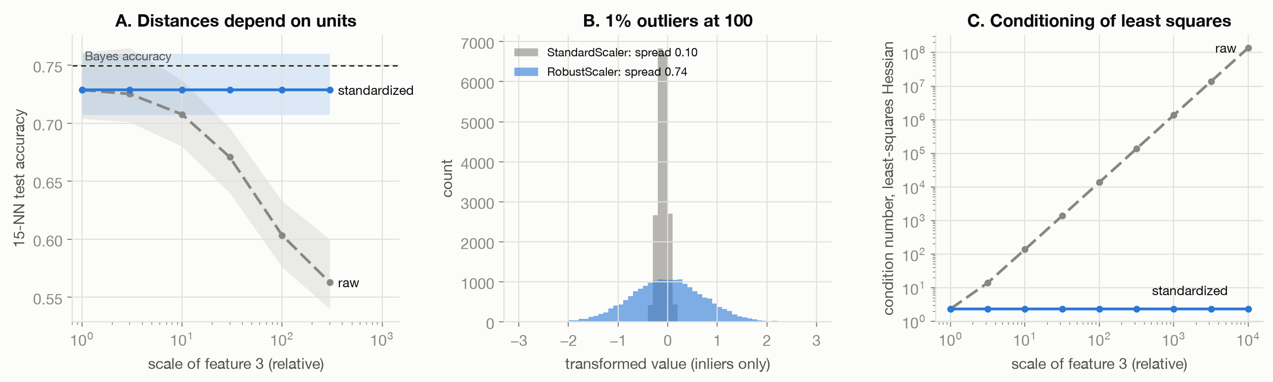
Figure 5.1 shows the three effects. The common failures:
- Using scaling to fix skew. It cannot; see the result above.
- Letting outliers choose the scale. Standard and min-max scaling compress the inliers when a few values are extreme. Robust scaling fixes the scale but leaves the outliers extreme. If they are errors, they should be fixed at the source (Cleaning).
- Equalizing what should not be equal. Standardization gives every feature the same spread, which means the same influence on distances. When one feature is known to matter more, that equality is itself an assumption.
5.6 What the toy cannot show
T1’s features are Gaussian or exactly log-normal, and the outliers are a clean 1% at one location. Real features mix units, have ties and gaps, and contain outliers at many scales. The demonstrations show which models are sensitive, not by how much on a given dataset.
5.7 Connections
- Cleaning: Missing Values, Duplicates, Outliers, Leakage: whether an extreme value is an error or a real tail case decides between removing it and scaling robustly.
- Changing the Shape: the nonlinear transforms that do change skew, and what they do to the target a model learns.
- optimization-lab, Foundations: why a large condition number slows gradient descent.
- Encoding and Features: encodings set the scale of categorical features, with the same consequences for distances and penalties.