15 A Data Decision Guide

Every chapter so far ended with a technique, the lever it pulls, the assumption it rests on and the way it fails. This chapter turns those cards into a procedure, then runs the procedure on two problems the book has not walked through: one tabular, one audio. Each step is checked against a known truth, which a real project never has. The table at the end lists every card.

15.1 The problem

Faced with a dataset and a model to train, which data techniques should be used, in what order, and how can each choice be checked before it is trusted?

15.2 Assumptions

The deployment question is known. What the predictions will be used for (a total, a ranking, a decision at a threshold) decides what “right” means. Without it, no step below can be checked.
Some data can be held out to check each step, split as deployment will be: by time for forecasts, by group for new groups, with duplicates removed across the split (Cleaning).
The worked examples use T1 and T5 (The Testbeds), so every check can be made against the exact answer.

15.3 Derivation or demonstration

The procedure. Four questions, asked in order. Each names a lever, and each lever has its own checks.

What will the model face, and what must it get right? Name \(p\), the deployment distribution, and the quantity the predictions must estimate: a conditional mean, a median, a probability at a given prior. Compare \(p\) with the data in hand, \(q\). Every gap between them is a reason for a technique, and the gap decides which (The Data-Generating Process, Distribution Shift).
Is the representation right for the model? For each input and for the target: does the model need the units, the shape, the order, or a structure the raw values hide? This is the representation lever (Data Types, Affine Scaling, Changing the Shape, Encoding and Features).
Does the training distribution match what the model must learn? If \(q\) differs from \(p\) in a known way, correct it by resampling, weights or augmentation: the \(q\) and \(w\) levers (Sampling and Weighting, Augmentation). If the labels are noisy, that is the label lever (Labels).
Is there enough data, and the right data? Fit a learning curve on a pilot, with an interval, and decide between more data, different data and a different model (Learning Curves, Choosing Data).

After each step, the check is the same: compare with a baseline that skips the step, on held-out data split as deployment will be, over several seeds. A technique whose assumption fails can make things worse, and only a comparison shows it.

Worked example 1: a skewed cost with a missing field (tabular). A team predicts a cost for each new case and adds the predictions up to plan a budget. The cost is positive and right-skewed. One field is missing in 35% of the training rows, more often when another field is large, because it was recorded only for some cases. New cases always have it. The data are T1 with log-normal noise of standard deviation 0.8 on the log scale, so the true conditional mean is known (20 seeds).

What must be right? The total, so each prediction must estimate \(\mathbb{E}[y \mid x]\), the conditional mean, not the median. The missingness depends on an observed field: missing at random (Cleaning).
Representation. A linear model on the raw cost cannot follow its exponential shape: the per-row relative error was 1.3. Least squares on \(\log y\), transformed back with \(\exp\), estimates the geometric mean, so the total came out -28% too low, as the derivation predicts (\(e^{-\sigma_\varepsilon^2/2} - 1\) = -27%). The smearing factor restored the mean: the total was off by -0.3% on average, between -7% and 5% across seeds, with a per-row error of 0.048 (Changing the Shape).
Training distribution. Dropping the incomplete rows selects on an observed field, which leaves \(p(y \mid x)\) unchanged (The Data-Generating Process): the numbers in step 2 are for complete cases. Mean imputation, by contrast, fills the field with a constant that ignores its correlation with the others; it shrank the fitted coefficients, and with smearing the total was still -13% off. Regression imputation kept the coefficients, but its imputed values carry no noise, so their error landed in the residuals that the smearing factor averages: the total was 3.8% too high (tests/test_worked_examples.py::test_regression_imputation_inflates_the_smearing_factor). The two corrections interact; checking each against a baseline is what shows it.
Enough data? With 2,000 rows, the total still varied by several percent from seed to seed; a learning curve on a pilot would say whether more rows narrow that spread (Learning Curves).

The whole example is one test (::test_cost_example_needs_smearing_and_the_right_missing_value_treatment).

Worked example 2: tones recorded at an unknown gain (audio). A device must tell two tones apart (400–600 Hz against 1,200–1,400 Hz, random phase, in noise) from a handful of labeled recordings made at one gain. Deployed devices record at gains up to 100 times higher or lower (±40 dB). The data are T5 (30 seeds).

What will it face? The same tones at other gains: a covariate shift whose effect on the input is known exactly. A gain multiplies tone and noise alike, so it adds the same constant, \(\log g\) for a gain \(g\), to every frequency of the log spectrum.
Representation. A linear model on the raw waveform was at chance (0.50), because the phase is random. The log spectrum drops the phase (Data Types). Trained on 10 recordings, it scored 0.98 at the training gain and 0.82 at the deployment gains.
Two fixes, two levers. Subtracting each recording’s mean log spectrum removes any gain exactly (::test_centering_the_log_spectrum_removes_any_gain_exactly): a representation fix, scoring 0.98. Augmenting each training recording with four copies at random gains, labels unchanged, teaches the same invariance through \(q\) (Augmentation): 0.98. The representation fix needs no extra training data; the augmentation needs no knowledge of how the gain acts, only that it does not change the label.
Enough data? With 100 recordings the plain log spectrum scored 1.000 at the deployment gains against 1.000 without the shift: here, more data alone also closes the gap (::test_tone_example_gain_shift_and_its_two_fixes).

Data card: Per-recording (per-sample) normalization

Changes	Representation (of \(x\)): each example is rescaled by a statistic of itself (here, its mean log spectrum is subtracted), not by statistics of the training set
Assumption	The nuisance acts on the whole example the same way (a recording gain scales every frequency alike), and the absolute level carries no information about the label
What it does to the learned function	Makes the features exactly invariant to the nuisance, so a shift in it at deployment cannot move the predictions
Which models care	Every model that sees the features; unlike per-feature scaling, it changes what even a tree can see
Fit on	Nothing: each example’s own values
Failure modes	The level does carry label information (loudness that matters is erased); the nuisance acts differently on different parts of the example (frequency-dependent gain is only partly removed)
Alternatives	Augmentation with random gains (teaches the invariance through \(q\)); per-feature scaling, which does not remove a per-example offset
Checked by	`tests/test_worked_examples.py::test_centering_the_log_spectrum_removes_any_gain_exactly`

Result: a procedure, not a recipe

Name the deployment distribution and the quantity to get right; fix the representation; match the training distribution to what must be learned; then ask whether there is enough data. Each step pulls one lever, rests on one assumption, and is checked against a baseline that skips it. In the tabular example the right target treatment depended on the missing-value treatment; in the audio example two levers fixed the same shift.

In practice

Write the deployment question down before touching the data. Change one thing at a time and keep the baseline that skips it. Report the spread across seeds or folds, not one number. When two techniques interact (a back-transform and an imputation; balancing and a threshold), check them together.

15.4 What it does to the learned model

A procedure does not change a model; the techniques it picks do, each through its lever. What the procedure adds is an account of why each technique is there, which assumption it rests on, and which check would show it failing. That account is what a reviewer, or a later version of the same team, needs when the deployment distribution moves.

15.5 Failure modes

Figure 15.1: Panel A: in the tabular example, the predicted total relative to the true total for each treatment of the missing field and of the skewed target (mean and range over 20 seeds); the dashed line is the derived bias of the plain back-transform. Panel B: the per-row relative error of the same pipelines and of least squares on the raw cost. Panel C: in the audio example, test accuracy against the number of training recordings when deployment gains vary by up to ±40 dB, for the raw waveform, the log spectrum, the centered log spectrum and the gain-augmented log spectrum, with the unshifted accuracy for reference (30 seeds). Each step of the procedure is checked against a truth: the skewed target needs smearing, the missing field a treatment that keeps \(p(y \mid x)\), and the gain shift a representation or an augmentation that removes it.

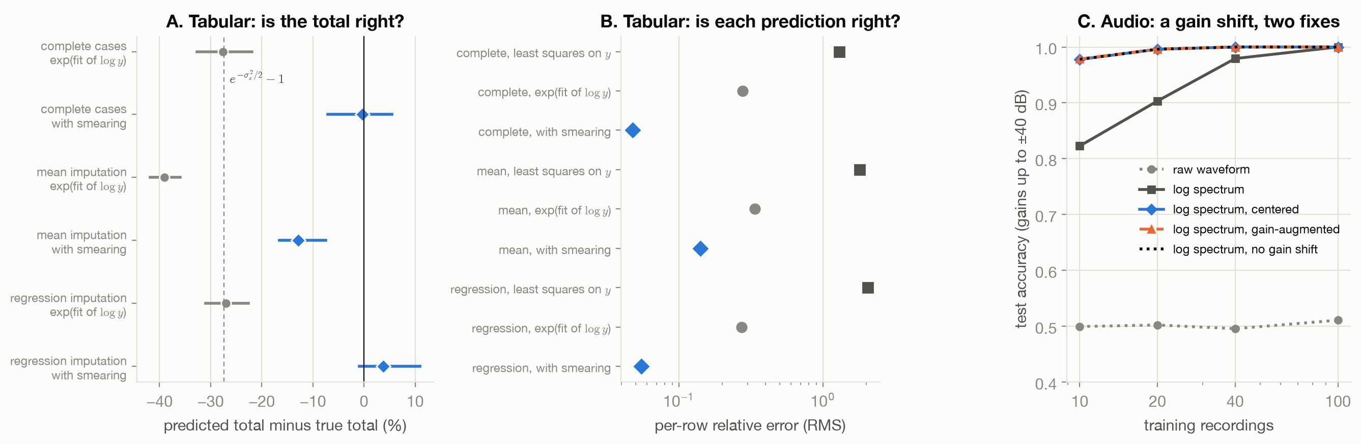
Figure 15.1 shows the checks. The failure modes of the procedure itself:

No deployment question. Without it, “the model is accurate” has no meaning: the plain back-transform is a fine median and a bad mean (panel A).
Checking techniques one at a time when they interact. Regression imputation and smearing are each sound alone, and together bias the total upward (panel A).
Judging by one metric. Least squares on the raw cost, with complete cases, missed the total by only -10% but got every row wrong (panel B).
Fixing a shift twice, or not at all. Centering and augmentation fix the same gain shift; using both adds cost, and using neither costs accuracy at small \(n\) (panel C).

15.6 What the toy cannot show

Here the truth is known, so every check is exact. In practice the checks use held-out data, which carries its own noise and its own shift, and the deployment question is often vague. Real tabular data has more fields, missing for less tidy reasons; real audio has noise, reverberation and gains that differ by frequency. The procedure transfers; the numbers do not.

15.7 Every data card

The table is generated from scripts/technique_data.py: one row per card, in chapter order.

Technique	Lever	Assumption	Fit on	Failure modes
Stratified sampling	Sampling distribution \(q\)	Strata are known for the whole population before sampling, and the target varies more between strata than within them	The population frame: stratum sizes	Strata unrelated to the target (no gain); disproportionate allocation without weights (biased estimates)
Finding label errors by confident learning	Labels	Class-conditional noise (flips independent of \(x\) given the true class); out-of-sample probabilities that rank examples well; classes that overlap little	Out-of-sample predictions (cross-validation), never the model’s own training fit	Overlapping classes: genuine ambiguity looks like noise (precision near the noise rate); flips near the boundary are missed; noise that depends on \(x\) breaks the assumption
Spectrogram (short-time Fourier magnitude)	Representation	The task depends on which frequencies are present and when, not on their phase; the window is long enough to resolve the frequencies that matter	None: a fixed transform (window length and overlap chosen in advance)	Window too short to resolve close frequencies or too long to localize changes in time; aliasing of frequencies above half the sampling rate happens before the transform and cannot be undone
Time-ordered evaluation splits	Evaluation only	Predictions will be made about later times than the training data; the series is autocorrelated or drifts	Split boundaries set by time stamps	Features computed over the whole series (rolling statistics, normalizers) still carry the future into the past; a single future window gives a noisy estimate
Complete-case analysis (dropping rows with missing values)	Sampling distribution \(q\)	For means and other summaries, MCAR: whether a value is missing is unrelated to anything. For a model of \(p(y \mid x)\), it is enough that missingness depends only on the model’s inputs	Nothing is fit; the selection is made by the missingness itself	MAR or MNAR missingness for summaries, and missingness that depends on the target for models (biased estimates); many columns with a little missingness each (few complete rows left)
Mean imputation	Representation	MCAR, and only the column’s mean matters downstream	Training rows only (the observed mean)	Non-MCAR missingness; heavy missingness (variance collapses); downstream use of variances or correlations
Regression imputation	Representation	MAR on the observed columns used as predictors, and a correctly specified imputation model	Training rows with the value observed	MNAR (the missing values differ in ways the predictors do not show); treating imputed values as observed
Removing train/test duplicates	Evaluation only	Deployment inputs will not be copies of training inputs	Exact (or near-duplicate) matching of test rows against training rows	Near-duplicates that exact matching misses; deployment that genuinely repeats inputs, where duplicates are part of \(p\)
Fitting preprocessing on training data only	Evaluation only	The evaluation should mimic deployment, where test labels and test inputs are not available at fit time	Training folds only (inside each cross-validation fold)	Steps fit outside the pipeline (feature selection, target encoding, resampling) before splitting
Affine scaling (standard, min-max, max-abs)	Representation	The model’s behavior depends on the features’ units; a feature’s typical spread is a fair yardstick for its importance	Training data only: mean and standard deviation, or minimum and maximum, or maximum absolute value	Outliers set the scale (standard and min-max); a feature that should matter more is made to matter equally; test values outside the training range (min-max)
Robust scaling (median and interquartile range)	Representation	Outliers are a small share of each feature (fewer than a quarter on each side)	Training data only: median and quartiles	Outliers are left in place at large values; features with an interquartile range of zero (mostly constant)
Log-transforming a skewed target	Representation	\(y > 0\), with multiplicative noise or right skew	None (a fixed function); the smearing correction is fit on training residuals	Retransformation bias; zeros and negatives; smearing fails when the log-scale noise depends on \(x\), and its factor is unstable when residuals are heavy-tailed
Box-Cox and Yeo-Johnson power transforms	Representation	Some power of the data is close to normal; Box-Cox needs strictly positive data, Yeo-Johnson does not	Training data only: \(\lambda\) by maximum likelihood	No power makes the data normal (multimodal data); \(\lambda\) estimated on few points is noisy; retransformation bias as for the log
Quantile transform	Representation	Only the order of values within a feature matters, not their spacing	Training data only: the quantiles of each feature	Distances lose their meaning (two values far apart in the tail become neighbors); no extrapolation: everything beyond the training range maps to the boundary
One-hot and ordinal encoding	Representation	One-hot: none about order; ordinal: the levels are ordered and the code’s spacing means something to the model	Training data only: the list of levels	Ordinal codes for unordered categories; unseen levels at test time; one-hot with very many levels (wide, sparse, rare columns)
Feature hashing	Representation	Collisions between levels are rare enough, or harmless enough, to accept for fixed memory	Nothing: the hash is fixed	Collisions grow with the number of levels: 2,000 levels in 1,024 columns use only about 880 of them; hashed columns cannot be traced back to levels
Target encoding	Representation	Levels with few rows are shrunk toward the global mean; each row’s encoding is computed without that row’s own label (cross-fitting)	Training labels, cross-fitted on the training rows (out-of-fold), and fit on all training rows for test data	Encoding training rows with an encoder fit on those same rows: noise becomes a training signal that fails on new data; leakage across a time order
Splines and discretization	Representation	The effect of \(x\) is smooth (splines) or roughly constant within intervals (bins); enough data per knot or bin	Training data only: knot or bin positions (quantiles or a uniform grid)	Too many knots or bins (variance); extrapolation beyond the training range; bins hide variation within an interval
TF-IDF	Representation	Word order does not matter for the task; terms common to every document carry little information	Training documents only: the vocabulary and document frequencies	Order and context are lost; rare terms are noisy; the vocabulary is fixed at fit time; the default token pattern drops one-character tokens
Rebalancing classes (undersampling or oversampling)	Sampling distribution \(q\)	Only the class priors change: \(q(x \mid y) = p(x \mid y)\)	Training labels (class counts)	Probabilities are wrong unless corrected; undersampling discards data and raises variance; oversampling by copying repeats examples
Class weights	Weights \(w\)	As for rebalancing: only the class priors are to be changed	Training labels (class counts); scikit-learn’s “balanced” uses n / (classes x count)	Probabilities are wrong unless corrected; very large weights on very rare classes make training noisy
Prior-shift correction (and EM prior estimation)	Weights \(w\)	Only the priors differ between training and target data; the model’s posteriors are calibrated under \(q\); for EM, the new data are unlabeled draws from the target	The training prior (counts) and the target prior (known, or estimated by EM on unlabeled target data)	\(p(x \mid y)\) also changed (not prior shift); miscalibrated training posteriors; EM converging slowly or to a biased value with few target examples
Importance weighting for covariate shift	Weights \(w\)	Covariate shift: \(p(y \mid x) = q(y \mid x)\); \(q(x) > 0\) wherever \(p(x) > 0\); the density ratio is known or well estimated	The density ratio: known here; in practice estimated, which adds its own error	Variance grows with \(\mathbb{E}_q[w^2]\), which grows exponentially with a Gaussian shift; regions where \(q\) is tiny dominate; an estimated ratio can be badly wrong where data is sparse
SMOTE (synthetic minority oversampling)	Sampling distribution \(q\)	The minority class occupies the space between nearby minority examples (locally convex); features are on comparable scales	Training minority examples only, inside each training fold	Minority clusters smaller than \(k\), or separated by majority regions: synthetic points land between clusters; noisy minority labels are interpolated; applied before the split it leaks
Label-preserving augmentation (flips, crops, color, SpecAugment, RandAugment)	Sampling distribution \(q\)	The target is invariant under the transform: \(p(y \mid T(x)) = p(y \mid x)\) for every transform \(T\) used, at the strengths used	Training data only, transformed during training	The invariance is false, or false beyond some strength: augmented examples are then mislabeled; test-time inputs never look like the augmented ones
Label-changing augmentation	Sampling distribution \(q\), Labels	The transform’s effect on the label is known exactly (here: a left-right flip reverses which half holds more ink)	Training data only	A wrongly assumed label change is label noise by construction; the effect may be known only for some inputs
mixup	Sampling distribution \(q\), Labels	Between two training examples, the target changes linearly along the segment joining them (a vicinal distribution around the data)	Training batches, with the mixing weight drawn from Beta(\(\alpha\), \(\alpha\))	Mixed inputs that are not plausible inputs; targets that are not linear between examples; small \(\alpha\) changes little, large \(\alpha\) blurs classes
Detecting shift with two-sample tests	Evaluation only	Samples within each period are i.i.d.; for input-only tests, the shift that matters shows up in \(p(x)\)	A reference sample from training time; for the classifier test, half of each sample (the other half is held out)	Concept shift leaves the inputs unchanged and is invisible to input-only tests; small shifts need large samples; a detected shift may not hurt the model, and an undetected one may
Estimating data needs from a pilot learning curve	Evaluation only	The fitted form holds beyond the pilot range; the pilot range already shows the asymptotic behavior; the floor \(C\) is identifiable from the pilot	The pilot data only, with train/test splits that never put copies of a row on both sides (bootstrap included)	The floor is poorly determined, so targets near it are often judged unreachable; the pre-asymptotic curve is steeper than the asymptote, so needed sizes are underestimated; intervals are wide
Coverage-driven selection	Sampling distribution \(q\)	What counts as covered can be recognized; unlabeled draws are cheap relative to labels or training steps	An unlabeled pool (or an oracle) and the record of what has been labeled	The gain is per label: it costs about \(n^{1+\alpha}\) unlabeled draws, and per draw nothing beats uniform sampling; a pool with fewer distinct cases than the labeling budget cannot spend it, and its error is that of the pool; recognizing coverage is trivial here and hard for real data (near-duplicates, semantic similarity)
Pruning by difficulty (keep hard or easy examples)	Sampling distribution \(q\)	The score ranks examples as the true margin would; the right end to keep depends on how much data there is	Scores from a probe model trained on the training data (a few epochs, or a different architecture)	Keeping hard examples with scarce data; noisy scores at high pruning rates, where random pruning can win (Ayed and Hayou); hard examples that are mislabeled
Deduplicating training data	Sampling distribution \(q\), Weights \(w\)	Repeats are artifacts of collection, not part of \(p\); what counts as a repeat (exact or near) can be defined	The whole corpus, before any split	Near-duplicates missed by exact matching; deduplicating genuine frequency information away; deduplicating after splitting
Active learning by uncertainty sampling	Sampling distribution \(q\)	Uncertainty reflects what the model has not learned, not irreducible label noise; the pool represents \(p\)	The labeled set so far and an unlabeled pool	Noisy labels: uncertainty points at noise, and the gain vanishes; the labeled set is no longer a sample of \(p\) (biased estimates); querying outliers
Training on model-generated data	Sampling distribution \(q\)	The generator’s distribution covers \(p\), including its tail	The generator’s own training data	Replacing real data generation after generation loses more of the tail each time; accumulating real and synthetic data does not
RHO-LOSS (reducible holdout loss selection)	Sampling distribution \(q\)	Holdout data from \(p\) is available; a small model’s loss estimates what is irreducible (noise) for each point	A holdout set, through the irreducible-loss model	A poor irreducible-loss model misjudges noise; holdout data that is not from \(p\)
Choosing domain mixtures (DoReMi)	Sampling distribution \(q\)	Weights found by a small proxy model transfer to a larger model	A small proxy model trained with group distributionally robust optimization over domains	Weights that do not transfer to the larger model or to the target task
Filtering web-scale data	Sampling distribution \(q\)	The filter’s notion of quality predicts usefulness for the target; enough data remains for the compute available	Heuristics or classifiers, sometimes trained on reference data	Filtering away rare but needed content (the tail); filtering choices that are right for one compute budget and wrong for another (Goyal et al.)
Per-recording (per-sample) normalization	Representation	The nuisance acts on the whole example the same way (a recording gain scales every frequency alike), and the absolute level carries no information about the label	Nothing: each example’s own values	The level does carry label information (loudness that matters is erased); the nuisance acts differently on different parts of the example (frequency-dependent gain is only partly removed)

15.8 Connections

The Map: the four levers and where each question of the book is answered.
Changing the Shape: the back-transform and smearing used in the tabular example.
Cleaning: the missing-value mechanisms behind step 3 of the same example.
Augmentation: invariance through \(q\), the second fix in the audio example.