13 Why Power Laws: The Long Tail
Scaling Laws reported that error falls as a power of the data, with exponents that simple theory does not predict. This chapter takes one explanation and makes it exact. When the cases a model must handle follow a long-tailed distribution, its error after \(n\) examples is the probability mass of the cases it has not yet seen. That mass shrinks as a power law, with an exponent set by the tail. The same exact model then answers a practical question: if most examples repeat what is already covered, can choosing examples do better, and better by what measure: per label, or per example drawn?
13.1 The problem
Why does each doubling of the data buy a smaller improvement? And could a smarter choice of which examples to label change that, or only shift it?
13.2 Assumptions
- Hutter’s toy model (Hutter 2021). Cases (“features”) \(i = 1, 2, \dots\) occur independently with probabilities \(p_i\). Each case has one fixed label, and the learner memorizes every case it has seen and errs on every other. Real learners generalize between cases; this one does not, which is what makes it exact. Hutter chose it over models that grow with the data and non-parametric models for simplicity, and notes that those routes should be pursued “since we have no indication that our findings transfer” (Hutter 2021, sec. 1).
- A Zipf tail: \(p_i = i^{-(\alpha+1)}/\zeta(\alpha+1)\) with \(\alpha > 0\). Word frequencies approximately follow such a law (Data Types and Their Structure). The values \(\alpha = 0.5, 1, 2\) used below are illustrative; none is a measured property of text.
- For selection, “covered” can be recognized. In the model a case is an exact identity; for real data, recognizing that two examples teach the same thing is itself hard.
13.3 Derivation or demonstration
Uniform sampling. A case is still unseen after \(n\) draws with probability \((1 - p_i)^n\), and it then costs its probability mass. So the expected error is Hutter’s eq. 2,
\[ E_n = \sum_i p_i\,(1 - p_i)^n , \]
and for the Zipf tail \(E_n \approx c\, n^{-\alpha/(1+\alpha)}\). The error is dominated by cases whose probability is about \(1/n\) (Hutter 2021, sec. 3). The testbed computes the sum exactly (The Testbeds). At \(\alpha = 1\), its local slope between \(10^5\) and \(10^6\) examples is -0.500 (tests/test_long_tail.py::test_learning_curve_slope_approaches_hutter_exponent).
Where the budget goes. By \(n = 100\) draws at \(\alpha = 1\), about 87% of draws were of cases already seen. Uniform sampling spends most of its budget on what is already covered. That explains why its exponent is small, but not why the error is a power law at all, as the next step shows.
The best any \(n\) labels can do. A memorizer that has labeled \(n\) distinct cases errs on the mass of the rest, and the \(n\) most frequent cases carry the most mass. So any \(n\) labels leave error at least the tail beyond them, \(E^{\text{oracle}}_n = \sum_{i>n} p_i\), which a selector reaches by labeling cases \(1, \dots, n\) in frequency order (tests/test_long_tail.py::test_any_n_labels_cost_at_least_the_tail_mass). Comparing the sum with an integral bounds it between \((n+1)^{-\alpha}\) and \(n^{-\alpha}\), each over \(\alpha\zeta(\alpha+1)\). Per label, the exponent rises from \(\alpha/(1+\alpha)\) to \(\alpha\): at \(\alpha = 1\), from -0.500 to -1.000. At 1,000 labels the error falls from 0.0218 to 0.00061 (::test_coverage_selection_beats_uniform_at_derived_rate). It is still a power law, because the tail is one.
Where the gain comes from. The oracle does two things: it never labels a repeat, and it labels frequent cases first. A selector that knows nothing of \(p\) can do the first. It reads the uniform stream and labels each case the first time it appears. After \(m\) draws it has used \(\mathbb{E}[D_m] = \sum_i 1 - (1-p_i)^m\) labels and its error is Hutter’s \(E_m\), both exact. Per label, its slope at \(\alpha = 1\) is -1.000, the oracle’s, and its error is 1.57 times the oracle’s. The same integral approximation that gives Hutter’s rate makes the factor \(\beta\,\Gamma(\beta)^{1+\alpha}\) with \(\beta = \alpha/(1+\alpha)\): \(\pi/2\) at \(\alpha = 1\), 1.46 at \(\alpha = 0.5\) and 1.66 at \(\alpha = 2\) (::test_deduplicated_stream_reaches_the_oracle_exponent_per_label; a simulation that stops at exactly 1,000 labels agrees within 2%, ::test_deduplicated_stream_exact_curve_matches_simulation). Not paying for repeats buys the exponent; knowing the frequency order adds only a constant.
What it costs. The gain is per label, not per draw. Reaching 1,000 labels this way took 524,000 draws at \(\alpha = 1\), close to the asymptotic count \((n/\Gamma(\beta))^{1+\alpha}\,\zeta(1+\alpha)\) derived in The Testbeds, which grows as \(n^{1+\alpha}\) (::test_deduplicated_stream_pays_n_to_the_one_plus_alpha_draws). Per draw, the error is still \(E_m\): nothing that reads a uniform stream does better than \(m^{-\alpha/(1+\alpha)}\) per example drawn. Coverage-driven selection pays off when labels (or training steps) are expensive and unlabeled draws are cheap.
On a long-tailed \(p\), a memorizing learner’s error is the mass of the cases it has not seen. Per example drawn it falls as \(n^{-\alpha/(1+\alpha)}\). Per label, no selection can beat the tail mass beyond \(n\), which falls as \(n^{-\alpha}\): a steeper power law, not an escape from one. Labeling only new cases reaches that exponent at a constant factor, and costs about \(n^{1+\alpha}\) draws.
This rate is not new. Michaud et al.’s quantization model uses the same Zipf form. A model that has learned the \(n\) most useful “quanta” has loss \(a + \frac{b-a}{\alpha\zeta(\alpha+1)}\,n^{-\alpha}\) (their eq. 2), the bound above. They read \(n\) as limited by model capacity, so their parameter exponent is \(\alpha\). With a threshold of examples per quantum, their data exponent is \(\alpha/(\alpha+1)\), Hutter’s (Michaud et al. 2023, sec. 2). In that reading, labeling only new cases reaches with \(n\) labels the rate that model size reaches with unlimited data.
| Changes | Sampling distribution \(q\): labels only examples that cover what is not yet covered (optionally most frequent first) instead of every draw from \(p\) |
| Assumption | What counts as covered can be recognized; unlabeled draws are cheap relative to labels or training steps |
| What it does to the learned function | On Hutter’s model the error per label falls as \(n^{-\alpha}\) instead of \(n^{-\alpha/(1+\alpha)}\): a steeper power law, still a power law. Skipping repeats buys the exponent; frequency order adds only a constant factor (about 1.5) |
| Which models care | Models that learn one case per example (memorization-like); the gain for models that generalize between cases is not measured here |
| Fit on | An unlabeled pool (or an oracle) and the record of what has been labeled |
| Failure modes | The gain is per label: it costs about \(n^{1+\alpha}\) unlabeled draws, and per draw nothing beats uniform sampling; a pool with fewer distinct cases than the labeling budget cannot spend it, and its error is that of the pool; recognizing coverage is trivial here and hard for real data (near-duplicates, semantic similarity) |
| Alternatives | Uniform sampling; active learning by model uncertainty; deduplication |
| Checked by | tests/test_long_tail.py::test_deduplicated_stream_reaches_the_oracle_exponent_per_label |
A selector with a finite pool. A realistic selector sees an unlabeled pool of \(M\) draws, ranks cases by how often they appear in it (ties broken at random), and labels the top \(n\). It cannot label a case absent from the pool, so its expected error is at least the larger of the oracle’s and the uniform error at the pool size, \(E_M\). This is the tail cut that Dohmatob et al. derive for a finite sample on the same model: \(T_0\) draws cut the tail near the case of probability \(1/T_0\) (Dohmatob et al. 2024, eq. 6 and Cor. 2.2). A pool often holds fewer distinct cases than the budget. With \(M = 10n\) and a budget of 1,000 labels, it held 138 on average; the selector labels them all, and its error is \(E_M\) exactly, the deduplicated stream after \(M\) draws (::test_small_pool_cannot_spend_its_budget). Measured against the budget, and so against the draws, its slope was -0.49, uniform sampling’s exponent (::test_linear_pool_keeps_the_uniform_exponent). Measured against the labels it used, it lies on the deduplicated stream’s curve (Figure 13.1, panel B). Only a pool large enough to hold more than \(n\) distinct cases, about \(n^{1+\alpha}\) draws, spends the budget and lets the ranking count: with \(M = n^{1+\alpha}\) the slope was -1.00, at 1.45 times the oracle’s error, against 1.57 for the deduplicated stream (::test_superlinear_pool_approaches_the_oracle_exponent).
Other accounts, and their scope. The long tail is one explanation of power-law scaling, not the only one:
- Data-manifold dimension (Sharma and Kaplan, 2020): parameter-scaling exponents near \(4/d\) arise from regression on a manifold of intrinsic dimension \(d\), with no tail (Sharma and Kaplan 2020, abstract).
- Variance- and resolution-limited regimes (Bahri et al., 2021): power laws arise from a well-behaved infinite-data limit, or from resolving a smooth manifold (Bahri et al. 2021, abstract).
- Memorization of rare subpopulations (Feldman, 2019, theory): when subpopulation frequencies are long-tailed, “memorization is necessary” for near-optimal generalization (Feldman 2019, abstract). This is the learning-theoretic face of the same tail.
- Long-tail knowledge in language models (Kandpal et al., 2022, one study): a model’s ability to answer a fact-based question “relates to how many documents associated with that question were seen during pre-training” (Kandpal et al. 2022, abstract).
- Spectral power laws (Maloney, Roberts and Sully, 2022, theory): in a solvable random-feature model, power laws in the data’s spectrum become power laws in the test loss, and the spectrum’s finite extent makes performance plateau (Maloney et al. 2022, abstract).
- Statistics of language (Cagnetta et al., 2026, one study): data-limited exponents predicted without free parameters from the decay of token correlations with distance and of next-token entropy with context length, matched to GPT-2- and LLaMA-style models on TinyStories and WikiText (Cagnetta et al. 2026, abstract).
Michaud et al. say they “tentatively find” that the frequencies of quanta in language models follow a power law matching the observed scaling exponent (Michaud et al. 2023, abstract). As of October 2026, which account dominates in a given system is an open question.
13.4 What it does to the learned model
Under a long tail, more data improves a model mostly at the edges: on cases it has never seen, which are individually rare and collectively common. That is why averages improve slowly while specific rare cases flip from wrong to right. It is also why removing redundancy (Choosing Data) and targeting the uncovered can change the curve, but only by changing which cases are covered, and only per label.
13.5 Failure modes
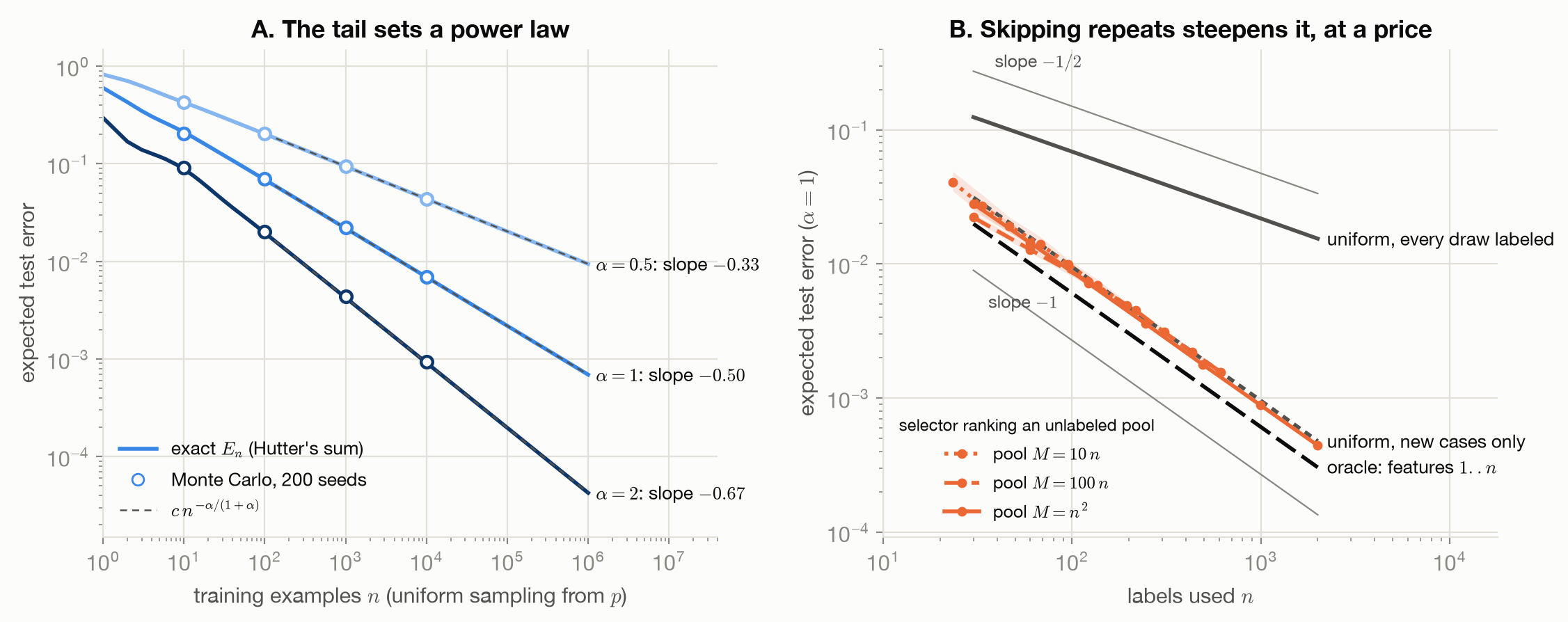
Figure 13.1 is the book’s signature figure. The failure modes it implies:
- Expecting selection to escape the power law. For a memorizing learner it changes the exponent per label, never below the tail mass beyond what was labeled.
- Counting labels, forgetting draws. The steeper curve per label costs about \(n^{1+\alpha}\) draws; per draw, nothing beats uniform sampling’s exponent.
- Selecting from a small pool. A pool with fewer distinct cases than the budget cannot spend it: its error is that of the pool, \(E_M\), whatever the budget.
- Mistaking redundancy for the cause. Redundancy slows uniform sampling; the tail makes the curve a power law. Remove all redundancy and the tail remains.
- Losing the tail. Training on data whose tail has been cut off, for example generated by a model, stops the curve at the cut. Dohmatob et al. derive the resulting plateau on this same model (Dohmatob et al. 2024), and Choosing Data reproduces it.
13.6 What the toy cannot show
The learner memorizes, the labels are deterministic, and cases are exact identities. Real models share structure between cases, so one example teaches about many, and “covered” is a matter of degree. The demonstration shows how a long tail can produce power-law returns, and what selection can and cannot buy when it does. It does not show that a given real scaling law arises this way.
13.7 Connections
- Scaling Laws: the empirical laws this chapter offers one mechanism for, and the alternative accounts.
- Learning Curves: a different source of diminishing returns (noise and dimension), with a floor instead of a tail.
- Choosing Data: deduplication, pruning and active learning, the practical forms of selection, and model collapse, the tail lost.
- Data Types and Their Structure: Zipf-like frequencies in text, the tail this model assumes.