4 Cleaning: Missing Values, Duplicates, Outliers, Leakage
Cleaning is usually presented as housekeeping: fill the gaps, drop the copies, clip the extremes, then get on with modeling. Each of those steps pulls a lever, though. Dropping rows changes the sampling distribution \(q\); filling a gap changes the representation; and the way a step is fit can change what an evaluation measures. This chapter derives what three common treatments of missing values do under each kind of missingness, then measures two leaks of very different size.
4.1 The problem
A dataset arrives with some values missing, some rows repeated, some values extreme, and a plan to fit preprocessing steps before the model. For each treatment, which quantities stay correct, and which become biased? The answer depends less on the treatment than on why the data looks the way it does.
4.2 Assumptions
- Missingness has a mechanism. Following Rubin (1976), van Buuren states the three cases this way: data are MCAR “if the probability of being missing is the same for all cases”, MAR “if the probability of being missing is the same only within groups defined by the observed data”, and MNAR if neither holds (Buuren 2018, sec. 1.2). Which case applies cannot be read off the observed data alone: it is an assumption about \(p\).
- One column goes missing, and a correlated column is always observed. With several incomplete columns the reasoning is the same, but the bookkeeping is not.
- Test examples will be new. Deployment does not show the model copies of its training rows. If it does (a lookup service, repeat customers), duplicates are part of \(p\), and removing them would be wrong.
4.3 Derivation or demonstration
Missing values. Consider column \(z_1\) of the tabular testbed, with true mean 0 and variance 1, 40% missing, and an always-observed column \(z_2\) correlated 0.6 with it. Three treatments:
- Complete-case analysis drops the rows where \(z_1\) is missing. It changes \(q\): the kept rows are a selection, and The Data-Generating Process showed what selection does.
- Mean imputation fills each gap with the observed mean. It changes the representation: a missing value is now encoded as an ordinary-looking number.
- Regression imputation fills each gap with the straight-line prediction from \(z_2\), fit on the rows where \(z_1\) is observed.
Under MCAR the kept rows are a random subset, so complete-case estimates are unbiased. Mean imputation keeps the mean but puts 40% of the values exactly at it. Its variance falls to about \(1 - r\) times the original, \(0.6\) here, with \(r\) the share imputed. Regression imputation keeps the part of the variance that \(z_2\) explains: imputed values have variance \(0.6^2\) of the original, so the total is \(1 - 0.4\,(1 - 0.6^2) = 0.744\). Over 200 seeds the measured variances were 0.995, 0.596 and 0.740.
Under MAR, here a missingness probability that rises with \(z_2\), the observed \(z_1\) values are skewed toward one side. Both the complete-case mean and the mean-imputed mean were \(-0.321\) on average. Regression imputation uses exactly the variable that drives the missingness, and its mean was \(-0.002\). Under MNAR, missingness rising with \(z_1\) itself, every treatment was biased. The best of the three was regression imputation, at \(-0.392\) (tests/test_missing.py::test_mcar_mean_imputation_shrinks_variance_mar_complete_case_biased).
A complete-case estimate of the mean is unbiased under MCAR, and biased here under MAR and MNAR. (Regressions fit to complete cases can stay unbiased when missingness depends only on the regression’s inputs: that is selection on \(x\), from The Data-Generating Process.) Mean imputation keeps the mean under MCAR only, and always shrinks the variance, by the share imputed. Regression imputation on the variables that drive the missingness removes the bias of the mean under MAR, but understates the variance. No treatment that uses only the observed data removes the bias under MNAR.
These match van Buuren’s summary of the same methods. Listwise deletion gives “unbiased estimates of means, variances and regression weights” under MCAR. Mean imputation will “underestimate the variance”. And under regression imputation “correlations are biased upwards, and the variability of the imputed data is systematically underestimated” (Buuren 2018, sec. 1.3). Multiple imputation, which adds the missing variability back by drawing several plausible values, is the standard remedy; it is beyond this book and Buuren (2018) treats it in full.
| Changes | Sampling distribution \(q\): keeps only rows whose value was observed |
| Assumption | For means and other summaries, MCAR: whether a value is missing is unrelated to anything. For a model of \(p(y \mid x)\), it is enough that missingness depends only on the model’s inputs |
| What it does to the learned function | Under MCAR, none beyond a smaller sample; under MAR or MNAR the kept rows follow a different distribution, so means shift, and so do fitted relationships unless the missingness depends only on the model’s inputs (selection on \(x\)) |
| Which models care | Every model |
| Fit on | Nothing is fit; the selection is made by the missingness itself |
| Failure modes | MAR or MNAR missingness for summaries, and missingness that depends on the target for models (biased estimates); many columns with a little missingness each (few complete rows left) |
| Alternatives | Regression or multiple imputation (MAR); modeling the missingness (MNAR) |
| Checked by | tests/test_missing.py::test_mcar_mean_imputation_shrinks_variance_mar_complete_case_biased |
| Changes | Representation: a missing value is encoded as the observed mean |
| Assumption | MCAR, and only the column’s mean matters downstream |
| What it does to the learned function | Keeps the mean under MCAR; shrinks the variance by the share imputed and weakens correlations; biases the mean under MAR or MNAR |
| Which models care | Linear and distance-based models see a spike at the mean; trees can split it off |
| Fit on | Training rows only (the observed mean) |
| Failure modes | Non-MCAR missingness; heavy missingness (variance collapses); downstream use of variances or correlations |
| Alternatives | Regression imputation; multiple imputation; a missing-indicator feature |
| Checked by | tests/test_missing.py::test_mcar_mean_imputation_shrinks_variance_mar_complete_case_biased |
| Changes | Representation: a missing value is encoded as its prediction from observed columns |
| Assumption | MAR on the observed columns used as predictors, and a correctly specified imputation model |
| What it does to the learned function | Removes the bias of the mean under MAR; still understates the variance (imputed values have no noise) and overstates correlations |
| Which models care | Every model; downstream uncertainty estimates are too narrow |
| Fit on | Training rows with the value observed |
| Failure modes | MNAR (the missing values differ in ways the predictors do not show); treating imputed values as observed |
| Alternatives | Multiple imputation, which adds the missing noise back (van Buuren); stochastic regression imputation |
| Checked by | tests/test_missing.py::test_mcar_mean_imputation_shrinks_variance_mar_complete_case_biased |
Duplicates. If some test rows are copies of training rows, a model that memorizes is rewarded twice. On T1, a 1-nearest-neighbor classifier trained on 2,000 rows scored 0.660 on 1,000 fresh test rows. With 30% of the test rows replaced by training rows, it scored 0.762, and with half, 0.830. The Bayes accuracy, the most any classifier can reach on new data, is 0.749. A test score above it is impossible on new data, so it measures memorization. On the fresh rows alone, the score stayed at 0.660 (20 seeds; tests/test_leakage.py::test_train_test_duplicates_inflate_the_test_score).
| Changes | Evaluation only: test rows that also appear in training are removed from the test set |
| Assumption | Deployment inputs will not be copies of training inputs |
| What it does to the learned function | None on the model; the test score stops rewarding memorization |
| Which models care | Most visible for models that can memorize (nearest neighbors, deep trees, large networks) |
| Fit on | Exact (or near-duplicate) matching of test rows against training rows |
| Failure modes | Near-duplicates that exact matching misses; deployment that genuinely repeats inputs, where duplicates are part of \(p\) |
| Alternatives | Group-aware splits (all copies of an entity on one side) |
| Checked by | tests/test_leakage.py::test_train_test_duplicates_inflate_the_test_score |
Leakage through fitted preprocessing. Kaufman et al. define leakage as “the introduction of information about the data mining target, which should not be legitimately available to mine from”. They separate leaking features from leakage in training examples (Kaufman et al. 2011, secs. 3.2–3.3). scikit-learn’s documentation gives the practical rule: never call fit on the test data. It says the risk applies to “almost all transformations in scikit-learn, including (but not limited to) StandardScaler, SimpleImputer, and PCA” (scikit-learn 1.9, Common pitfalls, §12.2).
The rule is right. The sizes of the two leaks it guards against are very different, though. On i.i.d. T1 data, a scaler, a min-max scaler or a mean imputer fit on train plus test instead of train alone changed test accuracy by at most 0.4 percentage points on average. That held for a 15-nearest-neighbor classifier and a strongly regularized logistic regression, over 200 seeds each. The changes were not consistently upward: the largest was \(-0.4\) points. These steps see the test inputs, whose distribution matches the training inputs, and never the test labels.
A supervised step is different. With 100 examples, 2,000 pure-noise features and labels that are coin flips, selecting the 20 features most associated with the labels on all the data, then cross-validating a classifier on them, reported an accuracy of 0.825. The same selection done inside each fold reported 0.513, close to the true 0.5 (20 seeds; tests/test_leakage.py::test_fitting_preprocessing_on_test_is_optimistic).
Fitting a step on the test data leaks what that step reads. An unsupervised step reads the test inputs, which on i.i.d. data carry little that the training inputs do not. A supervised step reads the test labels, and can fabricate a signal from noise.
| Changes | Evaluation only: every fitted step (scaler, imputer, selector, encoder) sees training data only |
| Assumption | The evaluation should mimic deployment, where test labels and test inputs are not available at fit time |
| What it does to the learned function | None on what the model can learn; removes optimism, which is large for supervised steps and small for unsupervised ones on i.i.d. data |
| Which models care | All |
| Fit on | Training folds only (inside each cross-validation fold) |
| Failure modes | Steps fit outside the pipeline (feature selection, target encoding, resampling) before splitting |
| Alternatives | A scikit-learn Pipeline cross-validated as one estimator |
| Checked by | tests/test_leakage.py::test_fitting_preprocessing_on_test_is_optimistic |
Put every fitted step in a sklearn.pipeline.Pipeline and cross-validate the pipeline as one estimator, so each step is refit inside each fold. scikit-learn 1.9’s SimpleImputer imputes the mean by default (strategy="mean"); add_indicator=True also appends a column marking which values were missing, which keeps the fact of missingness available to the model. That fact is itself informative whenever the data is not MCAR.
Outliers. An extreme value is either an error (a unit mix-up, a sensor fault) or a real case from the tail of \(p\). The two call for opposite treatments. Removing errors corrects the representation. Removing real tail cases changes \(q\) and teaches the model that the tail does not exist. No statistic separates them reliably, because both are, by definition, rare. Affine Scaling shows how one scaler is built to be insensitive to them, and robust losses are derived in loss-functions-lab.
4.4 What it does to the learned model
Missing-value treatments change the data a model is fit to in ways the model cannot detect. A mean-imputed column is a mixture of real values and a spike at the mean. A linear model fits a slope through both. A tree can split the spike off and use “was missing” as information, which under MAR or MNAR is real information. Complete-case analysis under MAR is selection: the model is fit to a distribution that differs from \(p\).
Duplicates and leaks change nothing about the model itself, only what we believe of it. Their cost appears later, when the deployed model performs as the fresh rows predicted, not as the contaminated test set promised.
4.5 Failure modes
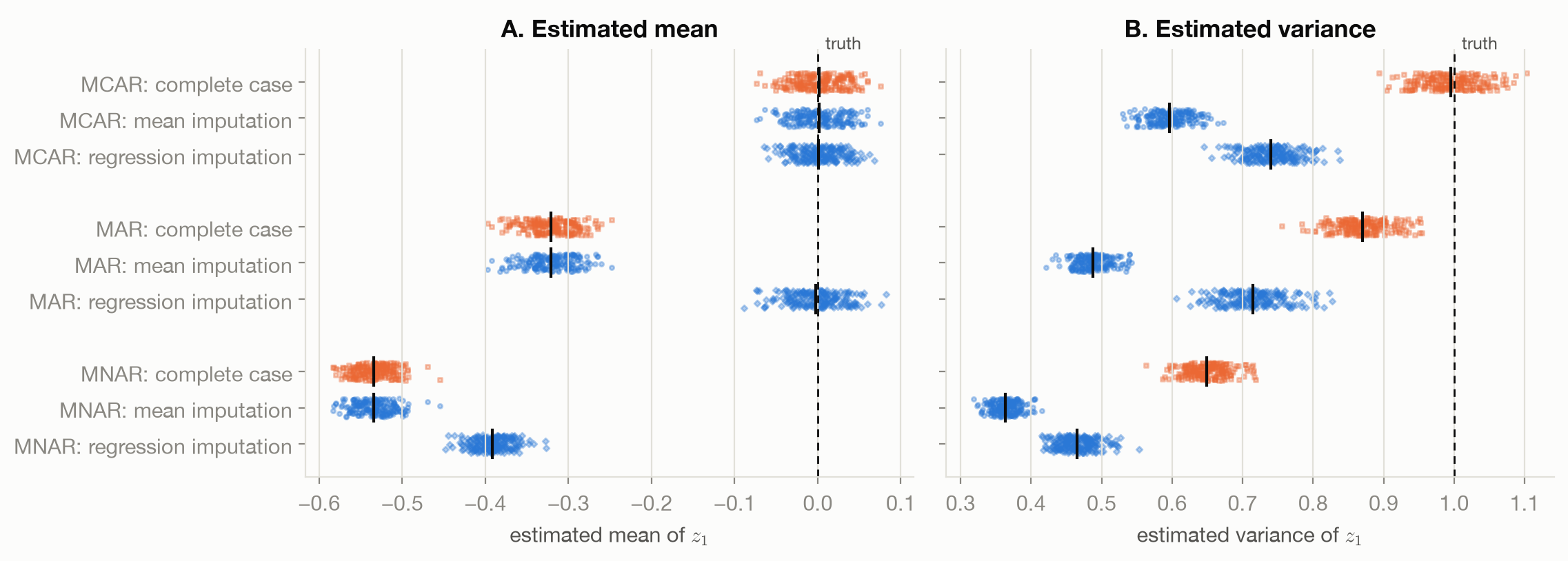
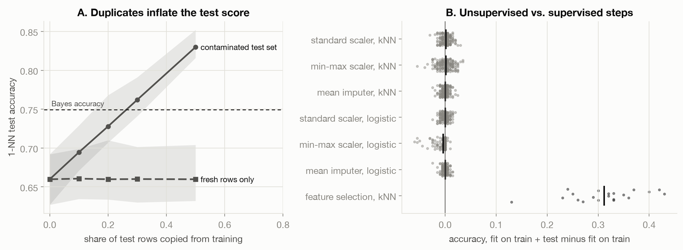
Figure 4.1 and Figure 4.2 show the failures measured above. Three more:
- Assuming MAR when the data is MNAR. Income goes unreported more often when it is high; a symptom goes unrecorded when it is absent. No observed column carries that dependence, so imputation from observed columns cannot remove it.
- Near-duplicates. Exact matching finds copied rows, not a resized image or a reformatted record. Choosing Data returns to deduplication at scale.
- Supervised steps hidden in “preprocessing”. Target encoding, feature selection by correlation, and resampling to balance classes all read the labels. Fit before the split, each is a leak of the second kind. Target encoding is the subject of Encoding and Features.
4.6 What the toy cannot show
The testbed’s missingness depends on one column through a known curve, and its duplicates are exact. Real missingness mixes mechanisms, and which one holds cannot be tested from the observed data. The demonstrations show what each treatment does under each mechanism, not which mechanism a real dataset has.
4.7 Connections
- The Data-Generating Process: complete-case analysis is selection, and the selection-on-\(x\) versus selection-on-\(y\) result applies.
- Data Types and Their Structure: temporal leakage is the ordered-data version of the leaks measured here.
- Affine Scaling: the next step after cleaning, and the first transform that is fit to the data.
- Encoding and Features: target encoding, the supervised preprocessing step that leaks most often in practice.