12 Scaling Laws
Learning Curves measured one model’s error as the data grew. Scaling laws make the same measurement across model sizes and compute budgets, at a scale where a single experiment costs millions, and fit simple formulas to the results. Those formulas now guide how training budgets are spent. This chapter states what the main studies report and how sure each result is. It then uses a source whose irreducible loss is known exactly to show what the fitted forms can and cannot tell you.
12.1 The problem
How does test loss fall as training data, model size and compute grow? How should a fixed compute budget be split between a larger model and more data? And what happens when the data runs out and has to be repeated?
12.2 Assumptions
- Symbols follow the cited papers in this chapter. \(D\) is a number of training tokens and \(N\) of parameters; \(E\), \(A\), \(B\), \(\alpha\) and \(\beta\) are Hoffmann et al.’s fitted constants, and \(\alpha_D\), \(\alpha_N\) Kaplan et al.’s exponents. They are not the book’s learning curve \(E_n\), Zipf exponent \(\alpha\) or dataset \(D\) (Notation).
- The results below are empirical. Unless stated otherwise, each is a finding of the cited study on its models and data, not a mathematical fact. Each is labeled with how widely it has been replicated, and dated.
- Loss is next-token cross-entropy, or test error, on held-out data from the training distribution. Downstream task performance can scale differently.
- For the demonstration, the model is a smoothed bigram model on T4. Its loss and the source’s entropy rate are exact; it has nothing to say about neural networks’ exponents.
12.3 Derivation or demonstration
Power laws in data (replicated finding). Hestness et al. measured how error falls with the training-set size across machine translation, language modeling, image recognition and speech. Their results “show power-law generalization error scaling across a breadth of factors”. Theory for simple settings predicts exponents of \(-0.5\) or \(-1\), but the measured exponent “usually settles between −0.07 and −0.35”, which the authors note is unexplained by prior theory (Hestness et al. 2017, sec. 1). Several groups have since reported power-law scaling. Rosenfeld et al. propose a functional form approximating error across both model and data scales (Rosenfeld et al. 2019, abstract only).
Language models (replicated, with contested details). Kaplan et al. report that, for transformers “trained with a limited dataset with early stopping”, the test loss follows \(L(D) = (D_c/D)^{\alpha_D}\) with \(\alpha_D \approx 0.095\) (their eq. 1.2). A matching law in the number of non-embedding parameters has \(\alpha_N \approx 0.076\) (eq. 1.1). Their compute-optimal allocation grows the model fastest, \(N \propto C^{0.73}\) (Kaplan et al. 2020, sec. 1).
Compute-optimal allocation (contested, as of October 2026). Hoffmann et al. trained over 400 models and concluded the opposite emphasis: “for compute-optimal training, the model size and the number of training tokens should be scaled equally: for every doubling of model size the number of training tokens should also be doubled” (Hoffmann et al. 2022, abstract). Their three estimation methods give exponents for \(N_{\text{opt}} \propto C^a\) of 0.50, 0.49 and 0.46 (their Table 2), against Kaplan et al.’s 0.73. They tested the prediction by training Chinchilla, a 70-billion-parameter model on 1.4 trillion tokens, which outperformed larger models trained on less data. Their third method fits
\[ \hat L(N, D) = E + \frac{A}{N^{\alpha}} + \frac{B}{D^{\beta}}, \]
where the first term “should correspond to the entropy of natural text”, and reports \(E = 1.69\), \(\alpha = 0.34\) and \(\beta = 0.28\) (Hoffmann et al. 2022, sec. 3.3 and Appendix D.2, eq. 10). A replication attempt of that third method found its estimates “inconsistent with their first two estimation methods” and its confidence intervals “implausibly narrow”; refitting gave results compatible with the first two methods (Besiroglu et al. 2024, abstract). The equal split itself has held up; the parametric fit has not.
Repeated data (single study, 2023). When unique data runs out, Muennighoff et al. find that “training with up to 4 epochs of repeated data yields negligible changes to loss compared to having unique data”, and that with more repetition “the value of adding compute eventually decays to zero”. Their fitted half-life of repeated data is about 16 epochs, beyond which “returns diminish extremely fast” (Muennighoff et al. 2023, abstract and §6).
Why the exponents differ by regime (theory, 2021). Bahri et al. identify “variance-limited and resolution-limited scaling behavior for both dataset and model size, for a total of four scaling regimes”. Variance-limited scaling “follows simply from the existence of a well-behaved infinite data or infinite width limit”. Resolution-limited scaling can be explained by models “resolving a smooth data manifold” (Bahri et al. 2021, abstract). A single curve can therefore pass through regimes with different exponents.
A demonstration with a known floor. On the Markov text source T4, a bigram model with add-\(k\) smoothing was trained on \(D\) tokens, from \(10^2\) to \(10^6\). Its exact cross-entropy (10 seeds) approached the source’s entropy rate, 2.350 nats per token, reaching 2.351 at \(10^6\). Its excess over that floor followed no single power law. The local log-log slope ranged from -0.39 to -0.09 below about 3,000 tokens and settled near -1.04 late, the variance-limited regime of a model of fixed size. Both published forms were then fitted on \(D \le 10^4\) and extrapolated to \(10^6\):
- a pure power law, Kaplan et al.’s data form: fitted exponent 0.026; predicted loss 2.228, below the entropy rate, which no model can reach;
- a power law plus an irreducible term, the data part of Hoffmann et al.’s form: fitted floor 2.406 and exponent 0.27; predicted loss 2.442, above the truth, because the early exponent is not the late one (
tests/test_scaling_laws.py::test_data_scaling_has_a_floor_and_regimes).
Several groups report that test loss falls as a power law in data, model size and compute, over many orders of magnitude, with exponents far from those of simple theory (replicated finding). A power law holds within a regime. A form without an irreducible term eventually predicts losses no model can reach, and an exponent fitted in one regime need not hold in the next. How to split compute between model and data is contested in its details (as of October 2026), though the equal-split conclusion has survived a replication.
Fit scaling curves with an irreducible term, over the regime you will extrapolate into, and report the interval, not only the fit. Before buying more unique data, check whether repeating the data you have, up to a few epochs, costs anything measurable.
12.4 What it does to the learned model
A scaling law describes models; it changes none. What it changes is a budget decision: how large a model to train, on how many tokens, for how many epochs. Those decisions inherit the law’s uncertainty. A wrong exponent, or a missing floor, misallocates a budget at exactly the scale where experiments are too expensive to repeat.
12.5 Failure modes
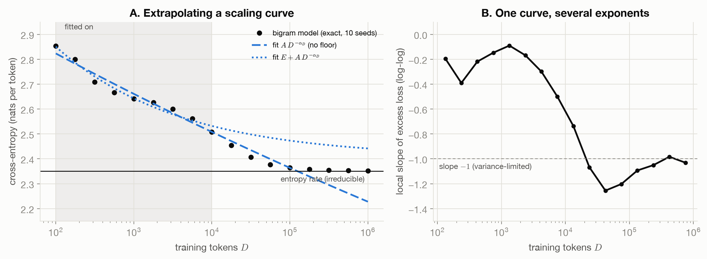
Figure 12.1 shows the demonstration. The failure modes:
- No floor in the formula. A pure power law always predicts that enough data drives loss to zero, and here below the entropy rate.
- Extrapolating across regimes. The fitted exponent belongs to the range fitted.
- Narrow intervals from few runs. The replication of Hoffmann et al.’s third method found intervals narrower than the number of experiments could support (Besiroglu et al. 2024).
- Confusing loss with capability. The laws above are about held-out loss on the training distribution; downstream behavior is a different measurement.
12.6 What the toy cannot show
A bigram model on a 50-token Markov source is not a transformer on natural text. Its exponents, regimes and crossover points are properties of the toy, not predictions about real models. What the toy does show is general: any curve with a floor bends away from a pure power law, and a fit on one regime misreads the next.
12.7 Connections
- Learning Curves: the same measurement at small scale, where the floor and pre-asymptotic bias were shown exactly.
- Why Power Laws: The Long Tail: a mechanism that produces power-law data scaling with a computable exponent.
- Choosing Data: repeated data, filtering and selection, the levers that try to change these curves rather than ride them.
- optimization-lab: “trained to convergence” and “early stopping” are optimization choices that the scaling laws above hold fixed.