6 Changing the Shape
Affine Scaling showed that the common scalers cannot touch a feature’s shape: a skewed feature stays skewed. Changing the shape takes a nonlinear transform: a log, a power, or a map through the feature’s own quantiles. These transforms change what the model sees. Applied to the target, they also change what a squared-error fit averages, and therefore what the model predicts once its output is transformed back. This chapter derives that change, measures how far the usual correction goes, and shows what the quantile transform gives up.
6.1 The problem
A price, an income or a waiting time is positive and right-skewed. Should it be transformed, and if it is the target, what does the prediction mean on the original scale? A model fit by squared error estimates a conditional mean, of whatever it was trained on (loss-functions-lab derives this). After a transform, that is the mean of the transformed target.
6.2 Assumptions
- The transform is strictly increasing, so it keeps the order of values and can be inverted. Every transform here is.
- For the log-target results, the noise is multiplicative and, on the log scale, independent of \(x\): \(\log y = m(x) + \varepsilon\), with \(\varepsilon\) independent of \(x\). If the noise’s spread depends on \(x\), the correction below breaks, and the chapter measures how.
- Box–Cox requires \(y > 0\). scikit-learn’s documentation says so plainly, and SciPy’s
boxcoxrejects non-positive input; a test confirms the rejection.
6.3 Derivation or demonstration
Shape, not scale. On 5,000 draws of a log-normal feature, the skewness is 7.05 raw, 7.05 after standardization, 0.06 after a log, and 0.00 after a quantile transform to a normal distribution (Figure 6.1, top row). The two nonlinear transforms reach the shape that no affine map can.
What squared error averages after a log. Fit \(\log y\) by least squares. The fit estimates \(\mathbb{E}[\log y \mid x] = m(x)\), so exponentiating the prediction estimates \(\exp(\mathbb{E}[\log y \mid x])\), the conditional geometric mean. When \(\varepsilon \sim \mathcal{N}(0, \sigma_\varepsilon^2)\), this is also the conditional median. The conditional mean is larger:
\[ \mathbb{E}[y \mid x] = \exp\big(m(x)\big)\, \mathbb{E}\big[e^{\varepsilon}\big] = \exp\big(m(x)\big)\, e^{\sigma_\varepsilon^2/2}. \]
The second equality is the log-normal mean, checked against SciPy’s log-normal distribution in the testbed’s tests. The naive back-transform therefore underestimates the mean by the factor \(e^{-\sigma_\varepsilon^2/2}\). With \(\sigma_\varepsilon = 0.8\) that factor is 0.726. On T1, the naive prediction averaged between 0.719 and 0.731 of the true conditional mean across 10 seeds, and 1.00 of the true geometric mean (tests/test_transforms.py::test_log_target_mse_predicts_geometric_mean).
The smearing correction. The middle expression above suggests the fix. Under assumption 2, \(\mathbb{E}[y \mid x] = \exp(m(x))\,\mathbb{E}[e^\varepsilon]\), and \(\mathbb{E}[e^\varepsilon]\) can be estimated without assuming a distribution, by averaging \(e^{\hat\varepsilon_i}\) over the training residuals. Duan proposed this smearing estimate as “a nonparametric estimate of the expected response on the untransformed scale after fitting a linear regression model on a transformed scale” (Duan 1983). Only that abstract could be read; the formula here is derived, not quoted. On T1 the smeared prediction averaged between 0.988 and 1.008 of the true mean across the 10 seeds.
Least squares on \(\log y\), transformed back with \(\exp\), estimates the conditional geometric mean (the median, for log-normal noise), not the conditional mean. Under log-normal noise of spread \(\sigma_\varepsilon\) the shortfall is the factor \(e^{-\sigma_\varepsilon^2/2}\). Smearing, which multiplies by the average of \(e^{\hat\varepsilon_i}\), restores the mean only if the log-scale noise does not depend on \(x\).
| Changes | Representation (of \(y\)) |
| Assumption | \(y > 0\), with multiplicative noise or right skew |
| What it does to the learned function | With MSE, the model learns \(\mathbb{E}[\log y \mid x]\): on the original scale, the geometric mean (the median under log-normal noise), not the mean |
| Which models care | Linear and GLM-type models, neural nets; trees much less |
| Fit on | None (a fixed function); the smearing correction is fit on training residuals |
| Failure modes | Retransformation bias; zeros and negatives; smearing fails when the log-scale noise depends on \(x\), and its factor is unstable when residuals are heavy-tailed |
| Alternatives | Box-Cox / Yeo-Johnson; a log-link GLM; a loss matched to the noise |
| Checked by | tests/test_transforms.py::test_log_target_mse_predicts_geometric_mean |
Power transforms. Box and Cox’s family replaces the log by a power that is chosen from the data (Box and Cox 1964). In SciPy’s notation it is \((y^\lambda - 1)/\lambda\) for \(\lambda \ne 0\) and \(\log y\) for \(\lambda = 0\), with \(\lambda\) chosen to maximize a profile log-likelihood (SciPy 1.18 docstrings of boxcox and boxcox_llf). A test builds positive data whose Box–Cox transform with a chosen \(\lambda\) is exactly normal, then estimates \(\lambda\) by maximum likelihood on 2,000 points. Over 50 seeds the mean estimate was \(-1.007\), \(-0.504\), \(-0.006\), \(0.495\) and \(1.486\) for true values \(-1\), \(-0.5\), \(0\), \(0.5\) and \(1.5\). scikit-learn’s PowerTransformer(method="box-cox") finds the same \(\lambda\) (tests/test_transforms.py::test_box_cox_mle_recovers_known_lambda).
Yeo and Johnson’s family extends the idea to zero and negative values (Yeo 2000). For \(x \ge 0\) it is the Box–Cox transform of \(x + 1\); negative values get a mirrored power with exponent \(2 - \lambda\) (SciPy 1.18, yeojohnson). A test confirms both properties and that the transform stays finite and increasing where Box–Cox fails (tests/test_transforms.py::test_yeo_johnson_extends_box_cox_to_zero_and_negative_values). It is scikit-learn’s default power transform.
| Changes | Representation: a power transform whose exponent \(\lambda\) is chosen by maximum likelihood to make the data as close to normal as the family allows |
| Assumption | Some power of the data is close to normal; Box-Cox needs strictly positive data, Yeo-Johnson does not |
| What it does to the learned function | Reduces skew; for a target, the model learns a mean on the transformed scale, which back-transforms to the median of \(y\) when the transformed noise is symmetric, not to the mean |
| Which models care | Linear, GLM-type and distance-based models; trees are unaffected (monotone) |
| Fit on | Training data only: \(\lambda\) by maximum likelihood |
| Failure modes | No power makes the data normal (multimodal data); \(\lambda\) estimated on few points is noisy; retransformation bias as for the log |
| Alternatives | A fixed log; a quantile transform; modeling the skew in the loss |
| Checked by | tests/test_transforms.py::test_box_cox_mle_recovers_known_lambda |
The quantile transform. Map each value through the feature’s estimated cumulative distribution function and the result is uniform; map that through \(\Phi^{-1}\) and it is normal. Every marginal shape becomes the chosen one. The price is the spacing. Ranks within each feature survive exactly (Spearman correlation 1), but distances do not. On log-normal data, the pairwise Euclidean distances after the transform correlated only 0.45 with those before. Any common rescaling would give exactly 1 (tests/test_transforms.py::test_quantile_transform_changes_distances_preserves_ranks). The scikit-learn documentation warns of the related effect on relationships: the transform “may distort linear correlations between variables measured at the same scale”.
| Changes | Representation: each feature is replaced by its estimated quantile, then mapped to a uniform or normal distribution |
| Assumption | Only the order of values within a feature matters, not their spacing |
| What it does to the learned function | Any marginal shape becomes the chosen one; ranks within a feature are kept, distances and linear correlations are not |
| Which models care | Distance-based and linear models change most; trees are unaffected on the training data (monotone) |
| Fit on | Training data only: the quantiles of each feature |
| Failure modes | Distances lose their meaning (two values far apart in the tail become neighbors); no extrapolation: everything beyond the training range maps to the boundary |
| Alternatives | A log or power transform, which keeps the spacing’s order of magnitude |
| Checked by | tests/test_transforms.py::test_quantile_transform_changes_distances_preserves_ranks |
PowerTransformer defaults to method="yeo-johnson" and standardize=True (scikit-learn 1.9). For a log target, sklearn.compose.TransformedTargetRegressor(func=np.log, inverse_func=np.exp) fits on \(\log y\) and back-transforms with \(\exp\): it returns the geometric mean, not the mean, unless the smearing factor is applied. QuantileTransformer uses n_quantiles=1000 and output_distribution="uniform" by default.
6.4 What it does to the learned model
A shape-changing transform on a feature changes which functions are simple. A relationship that is linear in \(\log x\) is a curve in \(x\), and a linear model can fit only one of them. On the target it changes the estimand itself. The model’s output, transformed back, is a different summary of the conditional distribution: a geometric mean or median instead of a mean. Whether that is a defect depends on the decision. Pricing a portfolio needs means, because totals are sums. Quoting a typical price can use medians.
6.5 Failure modes
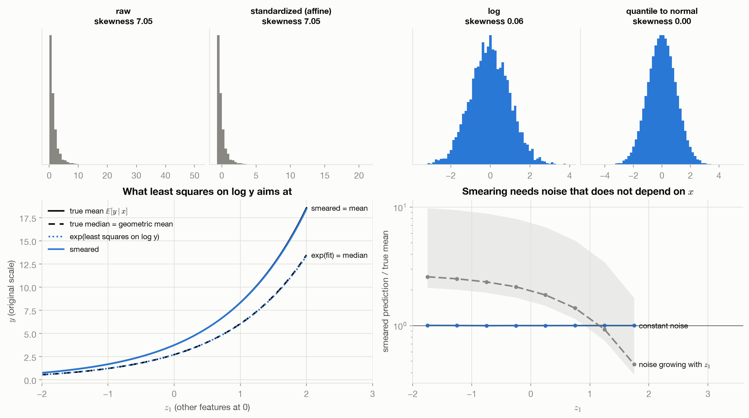
The main failure is the one assumption 2 rules out. Let the log-scale noise grow with \(z_1\) (\(\sigma_\varepsilon = 0.8\,e^{0.5 z_1}\)). One smearing factor is then too large where the noise is small and too small where it is large. Over 10 seeds, the smeared prediction’s ratio to the truth was 2.3 to 2.4 times higher for \(z_1 < -0.5\) than for \(z_1 > 0.5\). Worse, the factor itself, an average of exponentiated residuals, is dominated by the few largest. It ranged from 2.1 to 11.1 across seeds, against 1.37 to 1.38 with constant noise (tests/test_transforms.py::test_smearing_fails_under_heteroscedastic_noise). Three more:
- Zeros and negatives. The log and Box–Cox are undefined there. Adding a constant first changes the transform’s meaning near zero, and Yeo–Johnson’s \(x + 1\) is a specific choice of that constant.
- No extrapolation. A quantile transform maps every value beyond the training range to the boundary. Two new values, twice and a hundred times the training maximum, both map to exactly 1 (
tests/test_transforms.py::test_quantile_transform_clips_values_beyond_the_training_range). - Distances that no longer mean anything. After a quantile transform, two values far apart in the tail can become neighbors, which matters to every distance-based model.
6.6 What the toy cannot show
T1’s target is exactly log-normal, so the log is exactly right and the shortfall factor is known. Real targets are only roughly log-normal, and the right transform, if one exists, is unknown. The demonstrations show what each transform aims at and when its correction holds, not which transform to choose for a given dataset.
6.7 Connections
- Affine Scaling: the transforms that change units without changing shape.
- loss-functions-lab, Gaussian squared error: why squared error targets a conditional mean, the fact this chapter applies on a transformed scale.
- Encoding and Features: splines and discretization change shape too, by giving the model more flexible functions of a feature.
- Learning Curves: the noise level \(\sigma_\varepsilon\) that sets the retransformation gap also sets the floor of a regression learning curve.