1 The Data-Generating Process
A model is trained on the examples someone collected, and then used on the examples the world produces. When the two match, the gap between them is ordinary sampling noise, and more data closes it. When they do not match, more data makes the model more confident about the wrong thing. Every technique in this book is a deliberate change to what the model sees. This chapter is about the changes nobody chose: the ones made by how the data was gathered.
1.1 The problem
There are two distributions in every learning problem. The target distribution \(p(x, y)\) describes the cases the model will face once deployed. The training distribution \(q(x, y)\) describes the cases it was fit on. A model fit by minimizing average loss on a sample from \(q\) estimates the minimizer of the risk under \(q\). What we want is the risk under \(p\):
\[ R(\theta) = \mathbb{E}_{(x, y) \sim p}\big[\ell(y, f_\theta(x))\big]. \]
The question of this chapter is: when \(q\) differs from \(p\) because of how examples were collected, which part of what the model learns changes, and which part survives?
1.2 Assumptions
- The world produces examples from a fixed \(p\). If \(p\) itself moves over time, that is distribution shift, the subject of Distribution Shift.
- Collection keeps or drops each example with a probability \(s(x, y)\) that may depend on the input, the target, or both. If several examples are kept or dropped together (a whole hospital, a whole user), examples are no longer independent; the selection rule then acts on clusters, and the variance calculations below understate the noise.
- For the regression results, the model family contains \(p(y \mid x)\)’s conditional mean. If the model is misspecified, even selection on \(x\) changes which approximation is best, because it changes where the loss is averaged.
1.3 Derivation or demonstration
Suppose an example drawn from \(p\) is kept with probability \(s(x, y)\). Then the kept examples follow
\[ q(x, y) = \frac{s(x, y)\, p(x, y)}{\mathbb{E}_p[s(x, y)]}, \qquad q(y \mid x) = \frac{s(x, y)\, p(y \mid x)}{\int s(x, y')\, p(y' \mid x)\, dy'} . \]
If \(s\) depends on \(x\) only, it factors out of the integral and cancels:
If examples are selected with a probability that depends only on the input, the conditional distribution survives, \(q(y \mid x) = p(y \mid x)\), and only the input distribution changes: \(q(x) \propto s(x)\, p(x)\). If the probability depends on the target, \(q(y \mid x)\) differs from \(p(y \mid x)\), and no amount of data from \(q\) recovers it unless the selection probability \(s(x, y)\) itself is known.
This is a mathematical fact, and it splits selection into two very different cases. Selection on \(x\) changes the sampling distribution \(q\) over inputs: one of the four levers, and a lever that reweighting can undo when \(p(x)/q(x)\) is known (Sampling and Weighting). Selection on \(y\) changes what each input appears to say about its target, which is the same damage as corrupting labels.
Demonstration on T1. The tabular testbed (The Testbeds) draws \(\log y = a + b^\top z + \varepsilon\) with \(b_1 = 0.8\), three correlated features, and \(\mathbb{E}[\log y] = a = 1\). Each of 200 seeds draws 4,000 examples and keeps them in one of three ways:
- at random, half of them (\(q = p\));
- with probability \(\sigma(2 z_1)\), so large \(z_1\) is over-represented (selection on \(x\));
- with probability \(\sigma\big({-2}(\log y - \operatorname{median} \log y)\big)\), so large targets are under-represented, as when high values are less often recorded (selection on \(y\)).
A linear regression of \(\log y\) on \(z\) is then fit to the kept examples. Averaged over the 200 seeds, the coefficient on \(z_1\) is 0.802 under random selection and 0.801 under selection on \(x\): both are unbiased, as the result predicts. Under selection on \(y\) it is 0.670, a bias of about nine times the seed-to-seed standard deviation. The sample mean of \(\log y\) tells the opposite story. It is 1.00 under random selection, 1.45 under selection on \(x\) and 0.33 under selection on \(y\). Selection on \(x\) leaves the regression intact but biases any summary of the population (checked by tests/test_selection.py::test_selection_on_x_keeps_the_conditional_selection_on_y_biases_it).
When \(s(x, y)\) is known, as it is in the testbed, even selection on \(y\) can be undone. Since \(p \propto q / s\), weighting each kept example by \(1/s(x, y)\) restores the regression under \(p\). It does so slowly, because the rarest kept examples get the largest weights. The weighted coefficient was 0.781 with 4,000 examples per seed and 0.801 with 256,000, as the median largest weight grew from 64 to 478 (tests/test_selection.py::test_known_selection_probabilities_undo_selection_on_y). Real selection probabilities are almost never known, which is why the result box speaks of data from \(q\) alone.
Sampling designs. Some ways of drawing \(q\) are deliberate (Çetinkaya-Rundel and Hardin 2024, sec. 2.1.5):
- a simple random sample gives each case an equal chance of inclusion, with no case’s inclusion informative about another’s;
- a stratified sample divides the population into strata of similar cases, then samples within each stratum, usually at random;
- a cluster sample draws whole groups, keeping all their cases; a multistage sample draws groups and then samples within them;
- a convenience sample includes whoever is easy to reach, and “it is often difficult to discern what sub-population a convenience sample represents.”
Most machine-learning datasets are convenience samples: whatever was logged, scraped or labeled. Stratification is the one design here that is also a technique.
| Changes | Sampling distribution \(q\): fixes how many examples come from each stratum |
| Assumption | Strata are known for the whole population before sampling, and the target varies more between strata than within them |
| What it does to the learned function | None on \(q(y \mid x)\); with proportional allocation, \(q\) matches \(p\) on the strata exactly instead of on average, so estimates vary less |
| Which models care | Every model, through the variance of what it is fit on; most visible for rare strata |
| Fit on | The population frame: stratum sizes |
| Failure modes | Strata unrelated to the target (no gain); disproportionate allocation without weights (biased estimates) |
| Alternatives | Simple random sampling; post-stratification weights (\(w\)) |
| Checked by | tests/test_selection.py::test_stratified_sampling_lowers_the_variance_of_the_mean |
On T1, with four strata cut at the quartiles of \(z_1\) and samples of 200, a proportionally allocated stratified sample estimates the mean of \(\log y\) with 0.61 times the variance of a simple random sample. The prediction \(\sum_h W_h S_h^2 / S^2\) is 0.59, where \(W_h\) is a stratum’s share of the population, \(S_h^2\) its variance and \(S^2\) the overall variance (tests/test_selection.py::test_stratified_sampling_lowers_the_variance_of_the_mean).
sklearn.model_selection.train_test_split(..., stratify=labels) splits “in a stratified fashion, using this as the class labels” (scikit-learn 1.9 docstring). Stratifying a split by class keeps rare classes present in both halves. It does not make a convenience sample representative of anything.
1.4 What it does to the learned model
Selection on \(x\) changes where the model is accurate, not what it aims at. A flexible model fit to the kept examples still targets \(p(y \mid x)\), but it sees few examples where \(s(x)\) is small, so its estimate is noisy there and its errors concentrate there. A misspecified model does worse: it chooses the best approximation under \(q(x)\), which can be a poor approximation where \(p(x)\) puts its mass.
Selection on \(y\) changes the target itself. In the demonstration, the fitted line is flatter than the truth because large targets were removed more often where \(z_1\) is large, which pulls the high end down. The model is then miscalibrated over most of the range, and the error does not shrink with more data. It is a property of \(q\), not of the sample size.
1.5 Failure modes
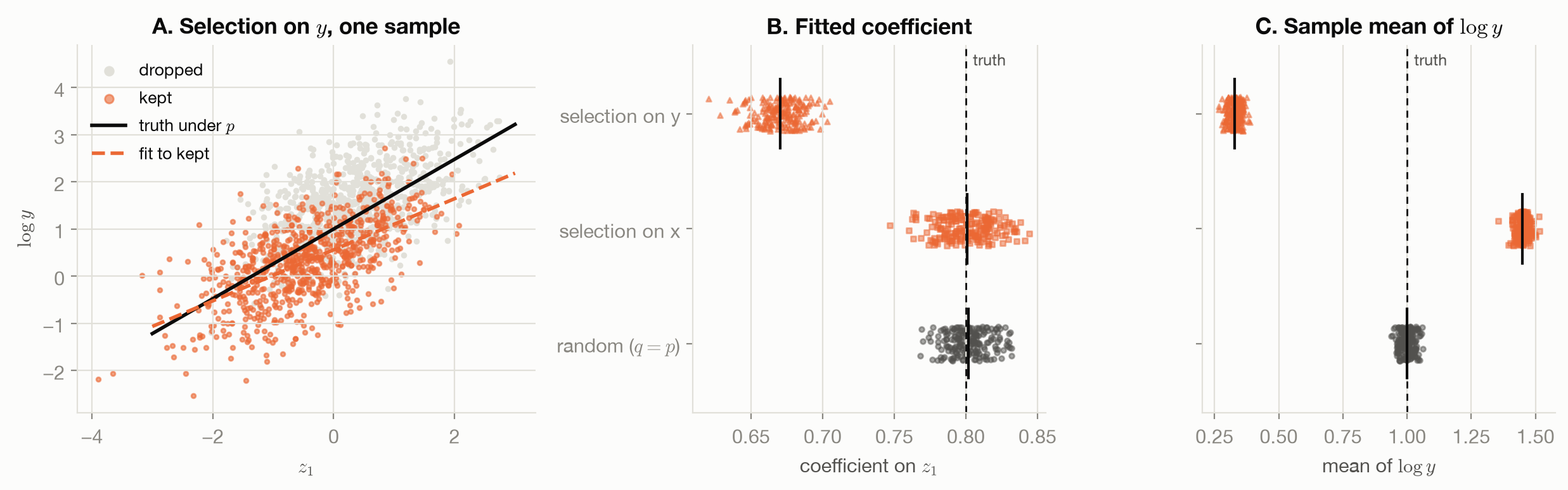
Figure 1.1 shows the two failures side by side. Three common forms:
- Outcome-dependent recording. Claims are filed only above a deductible; sensors saturate; a label is recorded only when someone complains. Each makes \(s\) depend on \(y\).
- Survivorship. The dataset contains only cases that lasted long enough to be observed, which again ties inclusion to the outcome.
- Undocumented convenience. Nobody recorded how examples were chosen, so nobody can tell which of the two cases applies. Datasheets were proposed against exactly this. Among the questions a dataset’s creators answer is whether it is “a sample (not necessarily random) of instances from a larger set”, and if so, whether it is representative (Gebru et al. 2018, sec. 3.2). A datasheet is the cheapest test for selection on \(y\) there is.
1.6 What the toy cannot show
T1 knows \(s(x, y)\) exactly. Real selection rules are rarely written down, usually depend on variables that are not in the dataset, and mix both cases. The demonstration also uses a correctly specified linear model. With a misspecified model, selection on \(x\) is no longer harmless, and how much it hurts depends on the model.
1.7 Connections
- Labels: selection on \(y\) and label noise both make \(q(y \mid x) \ne p(y \mid x)\); the next chapter treats the second.
- Sampling and Weighting: when selection depends on \(x\) alone and \(p(x)/q(x)\) is known, weighting each example by it restores the risk under \(p\).
- Distribution Shift: the same \(q \ne p\), caused by the world changing rather than by collection.
- rl-for-llms, Policy Gradients: the same pair, a sampling distribution \(q\) and weights \(w\), describes how reinforcement learning chooses its own data.