8 Sampling and Weighting
Part III turns from what each example looks like to which examples the model sees, and how much each one counts. Two levers do this: the sampling distribution \(q\) and the per-example weights \(w\). They are the same two levers that rl-for-llms uses to describe every policy-gradient method. Here they describe class rebalancing, prior correction, importance weighting and synthetic oversampling. This chapter derives what each one does to the learned probabilities, shows that resampling and reweighting aim at the same target, and measures what they cost.
8.1 The problem
A fraud detector trains on transactions in which 1 in 20 is fraud; a disease screen, on patients of whom few are sick. Common advice says to balance the classes: undersample the majority, weight the minority up, or synthesize minority examples. What does the model then learn, and does it still estimate the probability the deployment needs? And when the inputs seen in training differ from those met in deployment, can weights make up the difference?
8.2 Assumptions
- Prior shift. Rebalancing changes the class proportions and nothing else: \(q(x \mid y) = p(x \mid y)\). This holds when examples are chosen by their label only. Saerens et al. state this condition (Saerens et al. 2002, sec. 2.2), and it is what King and Zeng call choice-based sampling (King and Zeng 2001).
- Covariate shift. For importance weighting, inputs are drawn differently but labels follow the same rule, \(q(y \mid x) = p(y \mid x)\). Wherever \(p(x) > 0\), also \(q(x) > 0\), and the density ratio \(w(x) = p(x)/q(x)\) is known. The next chapter but one treats the case where it must be estimated.
- A well-specified, flexible enough model. The demonstrations use logistic regression on T1, whose true posterior is logistic, so differences come from the data, not the model.
8.3 Derivation or demonstration
What balancing does to the posterior. By Bayes’ rule, a model trained where class \(y\) has prior \(q(y)\) learns \(q(y \mid x) \propto p(x \mid y)\, q(y)\), while the target is \(p(y \mid x) \propto p(x \mid y)\, p(y)\). Under assumption 1 the likelihoods cancel in the ratio:
\[ p(y \mid x) = \frac{q(y \mid x)\, p(y)/q(y)}{\sum_{y'} q(y' \mid x)\, p(y')/q(y')}. \]
This is Saerens et al.’s eq. 4: the posterior under training conditions, “weighted by the ratio of the new priors to the old priors” and renormalized (Saerens et al. 2002). For a logistic model it reduces to King and Zeng’s prior correction: subtract \(\ln\big[\tfrac{1-\tau}{\tau}\,\tfrac{\bar y}{1-\bar y}\big]\) from the intercept, where \(\tau\) is the population fraction of ones and \(\bar y\) the sample’s (King and Zeng 2001, eq. 7). A test confirms that the two corrections agree to machine precision (tests/test_imbalance.py::test_king_zeng_intercept_correction_equals_saerens_for_logit).
On T1 with 5% positives (30 seeds, 20,000 examples each), a plain logistic regression’s predicted probabilities sat on average 0.0021 from the true posterior. Trained on a balanced undersample, the distance rose to 0.275; with balanced class weights, 0.276. After the correction from a training prior of 1/2 back to the true prior, the distances were 0.0034 and 0.0023 (tests/test_imbalance.py::test_prior_shift_correction_restores_calibration).
Training with class priors \(q(y)\) instead of \(p(y)\), by resampling or by weighting, makes the model learn \(q(y \mid x)\), the true posterior tilted by \(q(y)/p(y)\). Multiplying the output by \(p(y)/q(y)\) and renormalizing undoes the tilt exactly. At a threshold of 1/2, a model trained on balanced classes decides as the true posterior would at a threshold equal to the true prior (tests/test_imbalance.py::test_balanced_threshold_at_one_half_is_the_prior_threshold).
So “balance the classes” and “lower the threshold” are the same decision rule. The first changes the data and also destroys calibration; the second changes only the rule.
Same target, different variance. Undersampling pulls the \(q\) lever: it discards majority examples. Class weights pull the \(w\) lever: they keep every example and count the minority more. Both lead to the same tilted posterior. Over 30 seeds the coefficient on \(z_1\) averaged 1.500 with undersampling and 1.502 with weights; the truth is 1.5. Its standard deviation across seeds was 0.068 with undersampling and 0.048 with weights (tests/test_imbalance.py::test_resampling_and_reweighting_share_a_target_not_a_variance). The lever decides the variance, not the target.
| Changes | Sampling distribution \(q\): class proportions in training differ from those under \(p\) |
| Assumption | Only the class priors change: \(q(x \mid y) = p(x \mid y)\) |
| What it does to the learned function | The model learns the posterior tilted to the training priors; at threshold 1/2 a balanced model decides as the true posterior would at threshold \(p(y = 1)\) |
| Which models care | Every probabilistic classifier |
| Fit on | Training labels (class counts) |
| Failure modes | Probabilities are wrong unless corrected; undersampling discards data and raises variance; oversampling by copying repeats examples |
| Alternatives | Class weights (\(w\)); training on \(p\) and moving the threshold; prior-shift correction afterwards |
| Checked by | tests/test_imbalance.py::test_prior_shift_correction_restores_calibration |
| Changes | Weights \(w\): each example’s loss is multiplied by its class’s weight |
| Assumption | As for rebalancing: only the class priors are to be changed |
| What it does to the learned function | Same tilted posterior as resampling to the same proportions, with less variance because no example is discarded |
| Which models care | Every model trained by a weighted loss |
| Fit on | Training labels (class counts); scikit-learn’s “balanced” uses n / (classes x count) |
| Failure modes | Probabilities are wrong unless corrected; very large weights on very rare classes make training noisy |
| Alternatives | Resampling (\(q\)); moving the threshold; prior-shift correction |
| Checked by | tests/test_imbalance.py::test_resampling_and_reweighting_share_a_target_not_a_variance |
When the target prior is unknown. A model is deployed where the class mix has changed by an unknown amount. If only the prior changed, Saerens et al. estimate it from the unlabeled new data by EM. They start from the training prior, correct the posteriors to the current estimate with eq. 4, and set the next estimate to the corrected posteriors’ average (their eq. 9), until it stops moving. On T1, with a model trained at prior 0.5 and 5,000 unlabeled examples drawn at prior 0.1, the estimate averaged 0.1061 over 20 seeds and ranged from 0.089 to 0.139 (tests/test_imbalance.py::test_em_prior_estimation_recovers_test_prior).
| Changes | Weights \(w\) on the model’s output: each class’s posterior is multiplied by \(p(y)/q(y)\) and renormalized |
| Assumption | Only the priors differ between training and target data; the model’s posteriors are calibrated under \(q\); for EM, the new data are unlabeled draws from the target |
| What it does to the learned function | Turns posteriors learned under \(q\) into posteriors under \(p\); EM also estimates the unknown target prior |
| Which models care | Any classifier with calibrated probabilities |
| Fit on | The training prior (counts) and the target prior (known, or estimated by EM on unlabeled target data) |
| Failure modes | \(p(x \mid y)\) also changed (not prior shift); miscalibrated training posteriors; EM converging slowly or to a biased value with few target examples |
| Alternatives | Retraining on data from \(p\); recalibration on labeled target data |
| Checked by | tests/test_imbalance.py::test_em_prior_estimation_recovers_test_prior |
Importance weighting. Under covariate shift, labels follow the same rule but inputs are drawn from \(q\) instead of \(p\). Any average under \(p\) can then be written as a weighted average under \(q\):
\[ \mathbb{E}_{p}[\ell] = \mathbb{E}_{q}\big[w(x)\,\ell\big], \qquad w(x) = \frac{p(x)}{q(x)} . \]
The weighted sample mean is therefore unbiased. Its variance is \(\big(\mathbb{E}_q[w^2 \ell^2] - R^2\big)/n\), and \(\mathbb{E}_q[w^2]\) grows quickly with the shift. For Gaussian \(q = \mathcal{N}(0, \Sigma)\) and \(p = \mathcal{N}(\delta, \Sigma)\), it equals \(\exp(\delta^\top \Sigma^{-1} \delta)\). On T1, estimating the risk of a fixed classifier under \(p\) from 1,000 examples of \(q\), the weighted estimate was unbiased at every shift: at the largest, it averaged 0.096 against an exact 0.096. The unweighted estimate stayed at 0.250. The standard deviation of the weighted estimate grew from 0.014 to 0.039, as \(\mathbb{E}_q[w^2]\) grew from 1 to 104. The variance is known in closed form here, and its value lay inside the bootstrap interval of the measured variance at every shift (tests/test_shift.py::test_importance_weighting_unbiased_with_growing_variance).
Writing an average under \(p\) as a weighted average under \(q\) is importance sampling. Weighting a model’s training loss by \(p(x)/q(x)\) to correct covariate shift goes back at least to Shimodaira’s 2000 paper, whose title states the method: improving predictive inference under covariate shift by weighting the log-likelihood function [Shimodaira (2000); only its bibliographic record could be read for this book]. rl-for-llms uses the same pair \((q, w)\) for reinforcement learning (rl-for-llms, The Map).
| Changes | Weights \(w(x) = p(x)/q(x)\) on each training example’s loss |
| Assumption | Covariate shift: \(p(y \mid x) = q(y \mid x)\); \(q(x) > 0\) wherever \(p(x) > 0\); the density ratio is known or well estimated |
| What it does to the learned function | Weighted averages under \(q\) estimate averages under \(p\) without bias |
| Which models care | Any model trained or evaluated by an average loss |
| Fit on | The density ratio: known here; in practice estimated, which adds its own error |
| Failure modes | Variance grows with \(\mathbb{E}_q[w^2]\), which grows exponentially with a Gaussian shift; regions where \(q\) is tiny dominate; an estimated ratio can be badly wrong where data is sparse |
| Alternatives | Collecting data from \(p\); clipping or normalizing the weights (adds bias) |
| Checked by | tests/test_shift.py::test_importance_weighting_unbiased_with_growing_variance |
Synthetic minority examples. SMOTE oversamples the minority class by “taking each minority class sample and introducing synthetic examples along the line segments joining any/all of the k minority class nearest neighbors” (Chawla et al. 2002, sec. 4.2). Each synthetic point is a minority example plus a uniform fraction of the difference to one of its neighbors. It assumes the space between nearby minority examples belongs to the minority class.
| Changes | Sampling distribution \(q\): adds synthetic minority examples on segments between a minority example and one of its \(k\) nearest minority neighbors |
| Assumption | The minority class occupies the space between nearby minority examples (locally convex); features are on comparable scales |
| What it does to the learned function | More minority examples near existing ones; the minority region looks broader and smoother |
| Which models care | Models whose boundary depends on where minority examples lie (nearest neighbors, trees, kernels) |
| Fit on | Training minority examples only, inside each training fold |
| Failure modes | Minority clusters smaller than \(k\), or separated by majority regions: synthetic points land between clusters; noisy minority labels are interpolated; applied before the split it leaks |
| Alternatives | Class weights; random oversampling; prior-shift correction |
| Checked by | tests/test_imbalance.py::test_smote_fills_the_gap_when_k_exceeds_cluster_size |
scikit-learn’s class_weight="balanced" sets each class’s weight to n_samples / (n_classes * np.bincount(y)) (scikit-learn 1.9). The rebalanced model’s predict_proba is then tilted; correct it with the prior ratio, or keep the plain model and choose the threshold the decision needs. Resample or synthesize inside each training fold, never before splitting (Cleaning).
8.4 What it does to the learned model
Rebalancing does not teach the model anything new about the minority class. It changes the prior the model believes in. The ranking of examples, and hence any threshold-free metric, is unchanged in expectation. The probabilities are inflated by a known factor that can be removed. What rebalancing does change is the variance, through the lever used: discarding examples costs precision, and weighting does not.
Importance weighting changes the target from \(q\) to \(p\) at a price paid in effective sample size. At the largest shift here, 1,000 weighted examples estimate the risk under \(p\) about as precisely as 100 unweighted examples drawn from \(p\) itself would: the weighted estimate’s exact variance equals that of a plain average of about that many losses.
8.5 Failure modes
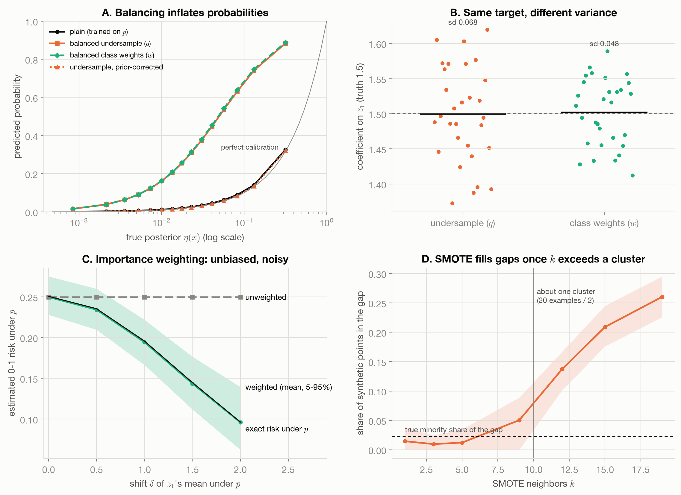
Figure 8.1 shows the four effects. The failure modes:
- Uncorrected probabilities. A rebalanced model used where probabilities matter (pricing, triage, combining with other evidence) overstates the minority class at every input (panel A).
- Weights that explode. Importance weights are heavy-tailed when \(q\) is thin where \(p\) is not. At the largest shift, the bootstrap interval for the estimator’s own variance spans a factor of 5.7 (panel C): even its precision is hard to measure. An estimated density ratio, which practice requires, adds its own error where data is sparse.
- SMOTE across gaps. With 20 minority examples split into two separated clusters, SMOTE with up to 5 neighbors put 1.2% of its synthetic points in the gap between them, against a true 2.3%. With 15 neighbors, more than a cluster holds, it put 20.9% there (
tests/test_imbalance.py::test_smote_fills_the_gap_when_k_exceeds_cluster_size). Those points are minority labels in majority territory. - A prior shift that is not one. If \(p(x \mid y)\) also changed (a new kind of fraud, not more of the old kind), eq. 4 and EM correct the wrong thing.
8.6 What the toy cannot show
T1’s posterior is exactly logistic, its density ratio is known in closed form, and its minority clusters are Gaussian. Real class-conditional distributions change along with the priors, density ratios must be estimated, and the geometry of a minority class is unknown. The demonstrations show what each lever targets and what it costs, not how well a given estimate of a prior or a ratio will work on real data.
8.7 Connections
- The Data-Generating Process: selection with a known probability is undone by the same \(1/s\) weights; importance weighting is that idea under covariate shift.
- Labels: the noisy-label posterior is also a known transform of the clean one, corrected by the same kind of algebra.
- Distribution Shift: how to tell covariate, prior and concept shift apart, and how to detect them.
- rl-for-llms, Policy Gradients: the same \((q, w)\) pair, where the learner chooses its own samples and weights them.