2 Policy Gradients
The previous chapter trained one policy three ways and ended each step with the same operation: a gradient step on \(\sum_i w_i\log\pi_\theta(y_i\mid x_i)\) over a batch of responses. That was not a coincidence of implementation. This chapter derives the policy gradient from scratch and shows that it is that operation. Maximizing expected reward produces a gradient that looks exactly like maximum-likelihood training, except that the responses are ones the model sampled itself and each one carries a weight that can be negative. This is the book’s second thesis and the single most useful identity in it: almost every post-training method, from SFT to PPO to DPO, can be written as a choice of which responses and what weight on each. The second half of the chapter deals with the price of sampling: the gradient estimate is noisy, and baselines, advantages and critics are the classical tools for living with that noise.
2.1 The problem
A policy \(\pi_\theta(y\mid x)\) produces a response \(y\) to a prompt \(x\), and a reward function \(r(x,y)\) scores it. The goal is to maximize the expected reward,
\[ J(\theta) = \mathbb{E}_{x\sim\mathcal{D}_x}\,\mathbb{E}_{y\sim\pi_\theta(\cdot\mid x)}\big[r(x,y)\big]. \]
Two features make this different from minimizing a supervised loss. First, the reward is a black box: it may be a rule-based checker, a human judgment or another network, and it need not be differentiable in \(y\). Even if it were, \(y\) is a sequence of discrete tokens, so there is no gradient to pass through it. Second, \(\theta\) enters \(J\) only through the distribution the expectation is taken over. Changing \(\theta\) does not change any response; it changes which responses are likely. The question is how to differentiate an expectation with respect to the parameters of the distribution it is taken over, using only samples and reward evaluations.
2.2 Assumptions
- The policy is differentiable and has full support where it matters. \(\nabla_\theta\log\pi_\theta(y\mid x)\) exists, and \(\pi_\theta(y\mid x) > 0\) for responses we want gradients for. A softmax over the next token guarantees both. If the policy assigned exactly zero probability to good responses it could never sample them, and the gradient would never point toward them.
- We can sample from the current policy and evaluate the reward on the samples. Nothing is assumed about the reward’s form.
- Expectations and gradients can be exchanged. True for the finite response spaces of language models (sums, not integrals).
2.3 Derivation
The one-step (bandit) case
Fix a prompt \(x\) and drop it from the notation. Write the expectation as a sum and differentiate:
\[ \nabla_\theta J = \nabla_\theta\sum_y \pi_\theta(y)\,r(y) = \sum_y r(y)\,\nabla_\theta\pi_\theta(y). \]
This is not yet usable, because \(\sum_y r(y)\nabla_\theta\pi_\theta(y)\) is not an expectation under anything we can sample from. The log-derivative trick makes it one. Since \(\nabla_\theta\log\pi_\theta(y) = \nabla_\theta\pi_\theta(y)/\pi_\theta(y)\), multiply and divide by \(\pi_\theta(y)\):
\[ \nabla_\theta J = \sum_y \pi_\theta(y)\,r(y)\,\nabla_\theta\log\pi_\theta(y) = \mathbb{E}_{y\sim\pi_\theta}\big[\,r(y)\,\nabla_\theta\log\pi_\theta(y)\,\big]. \]
Now the gradient is an expectation under the policy itself. Sample \(y_1,\dots,y_n\) from \(\pi_\theta\), evaluate their rewards, and average \(r(y_i)\nabla_\theta\log\pi_\theta(y_i)\). The average is an unbiased estimate of \(\nabla_\theta J\). The reward is never differentiated; it only multiplies. This estimator is Williams’s REINFORCE (Williams 1992), also called the score-function estimator, since \(\nabla_\theta\log\pi_\theta\) is the score of the policy.
The sequential case
A language model generates \(y = (y_1,\dots,y_T)\) one token at a time, so by the chain rule \(\pi_\theta(y\mid x) = \prod_t\pi_\theta(y_t\mid s_t)\), where \(s_t = (x, y_{<t})\) is the state before token \(t\). The log turns the product into a sum,
\[ \nabla_\theta\log\pi_\theta(y\mid x) = \sum_{t=1}^{T}\nabla_\theta\log\pi_\theta(y_t\mid s_t), \]
and nothing else in the derivation changes. Two things are worth noticing. The transition from \(s_t\) to \(s_{t+1}\) never appears, because in general the environment’s transition probabilities do not depend on \(\theta\) and drop out of \(\nabla_\theta\log\) of the trajectory’s probability; for text generation the transition is deterministic anyway (“append the token”). And with one reward at the end, every token’s score is multiplied by the same scalar \(r(x,y)\). In MDPs with rewards along the way, the reward-to-go \(G_t\) replaces \(r\) at step \(t\), because an action cannot affect rewards that came before it. That is the general policy gradient theorem, in the Monte Carlo (REINFORCE) form derived by Sutton and Barto (Sutton and Barto 2018, secs. 13.2–13.3):
\[ \nabla_\theta J = \mathbb{E}_{\pi_\theta}\Big[\sum_t G_t\,\nabla_\theta\log\pi_\theta(a_t\mid s_t)\Big]. \]
The climax: put the SFT gradient next to it
Supervised fine-tuning maximizes the log-likelihood of demonstrations \((x,y)\sim\mathcal{D}\). Its gradient is
\[ \nabla_\theta\mathcal{L}_{\text{SFT}} = \mathbb{E}_{(x,y)\sim\mathcal{D}}\big[\,1\cdot\nabla_\theta\log\pi_\theta(y\mid x)\,\big], \]
and the policy gradient is
\[ \nabla_\theta J = \mathbb{E}_{x\sim\mathcal{D}_x,\;y\sim\pi_\theta(\cdot\mid x)}\big[\,r(x,y)\cdot\nabla_\theta\log\pi_\theta(y\mid x)\,\big]. \]
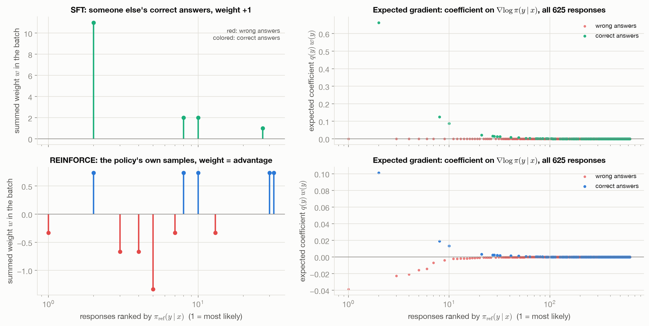
These are the same operation. Each pushes up the log-probability of some sequences. They differ in exactly two places: which sequences are used (a fixed dataset vs. the model’s own samples) and how much weight each one gets (always 1 vs. a reward that, after the baselines of the next section, can be negative and push a sequence down).
Figure 2.1 shows this on the toy language, for a prompt that \(\pi_{\text{ref}}\) answers correctly 19% of the time. On the left are actual batches: SFT sees 16 demonstrations, all correct and all weighted \(+1\); REINFORCE sees 16 of the policy’s own samples, and the correct ones get positive weight while the wrong ones get negative weight. On the right is the expected coefficient that each method puts on each response’s \(\nabla_\theta\log\pi_\theta(y)\), computed exactly for all 625 responses. SFT puts weight only on correct answers, in proportion to the expert’s probability for them, wherever they sit in the policy’s ranking. REINFORCE puts positive weight on correct answers in proportion to how likely the policy already finds them, and an equal total of negative weight on the wrong answers it currently favors. The most likely response under \(\pi_{\text{ref}}\) is wrong, so it receives the largest push down.
The \((q, w)\) form
The comparison generalizes into the frame for the rest of the book.
\[ \nabla_\theta\mathcal{J} \;=\; \mathbb{E}_{x\sim\mathcal{D}_x,\;y\sim q(\cdot\mid x)}\Big[\,w(x,y)\,\nabla_\theta\log\pi_\theta(y\mid x)\,\Big] \;+\; \text{(regularizer gradient)} \] A method is specified by its sampling distribution \(q\) (where the trained-on responses come from) and its per-sample weight \(w\) (or per-token weight \(w_t\) on \(\nabla_\theta\log\pi_\theta(y_t\mid s_t)\)). SFT: $q = $ the data, \(w = 1\). REINFORCE: \(q = \pi_\theta\), \(w = r\) (or an advantage).
This is not this book’s invention. Shao et al. make the same observation in the DeepSeekMath paper, writing the gradient of every method they study as an expectation over a data source of a gradient coefficient times \(\nabla_\theta\log\pi_\theta\), with the coefficient determined by a reward function and an algorithm, and they tabulate SFT, rejection-sampling fine-tuning, DPO, PPO and GRPO in those terms (Shao et al. 2024, sec. 5.2). In the toy implementation the form is literal: every method in rl4llm.methods ends in the same call, grad_log_likelihood(lang, logits, prompts, responses, weights), and differs only in the responses it passes and the weights it computes.
| Signal | scalar reward per response |
| Samples from (\(q\)) | \(\pi_\theta\), fresh samples every update (on-policy) |
| Per-sample weight (\(w\)) | the reward \(r(x,y)\), or \(r - b\) with a baseline |
| Stability | none beyond a small learning rate |
| Credit granularity | sequence level: the same weight on every token’s score (reward-to-go \(G_t\) per step in general MDPs) |
| Models in memory | policy (+ reward function) |
| Targets | \(\max_\theta\mathbb{E}_{\pi_\theta}[r]\), an unregularized objective |
| Classical lineage | Williams (1992); the Monte Carlo policy gradient (Sutton & Barto §13.3) |
2.4 Interpretation
What does following this gradient produce? It maximizes expected reward and nothing else. The weight on each response is its reward, so mass flows toward whatever the reward function scores highest. Nothing in the objective asks the policy to stay diverse or to stay close to where it started. The previous chapter showed the consequence: with a 0/1 correctness reward, REINFORCE ended with essentially all its probability on one correct answer, where SFT on the same task kept the expert’s spread. The KL penalty that every LLM recipe adds, and the closed-form optimum it produces, are the subject of the chapter on keeping updates stable and the shared-target chapter. Before that, there is a more immediate problem.
2.5 Variance, baselines and advantages
The estimator is unbiased, but a single sample tells you very little. Every response’s score is scaled by its reward, so the estimate depends on the reward’s level, not just on which responses are better. If all rewards are shifted up by 10, every sampled response gets pushed up hard; the gradient is still right on average, because the pushes on likely responses cancel in expectation, but each individual estimate is dominated by noise.
Why subtracting a baseline does not bias the gradient
The score function has mean zero:
\[ \mathbb{E}_{y\sim\pi_\theta}\big[\nabla_\theta\log\pi_\theta(y)\big] = \sum_y\nabla_\theta\pi_\theta(y) = \nabla_\theta\sum_y\pi_\theta(y) = \nabla_\theta 1 = 0. \]
So for any \(b\) that does not depend on the sampled response, \(\mathbb{E}[(r(y)-b)\nabla_\theta\log\pi_\theta(y)] = \mathbb{E}[r(y)\nabla_\theta\log\pi_\theta(y)]\). Subtracting a baseline changes nothing in expectation and can change the variance a great deal. Sutton and Barto note that the baseline “can be any function, even a random variable, as long as it does not vary with” the action (Sutton and Barto 2018, sec. 13.4). That condition is the whole design space of baselines, and it explains each common choice.
- A constant or running mean. Unbiased. Removes the reward’s overall level.
- A per-prompt value \(V(x) = \mathbb{E}_{\pi_\theta}[r\mid x]\). Unbiased. In a prompt where every answer scores well, only answers better than usual get pushed up.
- A learned critic \(V_\phi(s_t)\), per token. Unbiased as long as it depends only on the state, not on the token chosen there. This is the actor–critic architecture, and \(r - V_\phi(s_t)\) is an estimate of the advantage \(A(s_t,y_t)\) from the previous chapter.
- Leave-one-out (RLOO). Sample \(G\) responses for the same prompt and use, for response \(i\), the mean reward of the other \(G-1\): \(b_i = \frac{1}{G-1}\sum_{j\ne i}r_j\). Because \(b_i\) is built from samples independent of \(y_i\), it is unbiased, and it costs nothing beyond the extra samples. Kool, van Hoof and Welling proposed it under the memorable title “Buy 4 REINFORCE samples, get a baseline for free!” (Kool et al. 2019), and Ahmadian et al. brought it to RLHF (Ahmadian et al. 2024).
- The group mean including the sample itself. Biased: \(r_i\) appears in its own baseline with weight \(1/G\), so the expected gradient is shrunk by \((G-1)/G\). Rescaling by \(G/(G-1)\) turns it exactly into RLOO.
- The group mean and standard deviation (GRPO). Divides each prompt’s centered rewards by that prompt’s reward standard deviation. This is no longer only a baseline: it rescales different prompts differently and so changes which objective is being followed. Policy Gradients Without a Critic takes it apart.
The baseline was already in Williams’s original work (Sutton and Barto 2018, sec. 13.4 notes). RLOO and GRPO’s group mean are Monte Carlo baselines: estimates of \(V(x)\) built from extra samples instead of a learned network. A learned \(V_\phi(s_t)\) is the critic of actor–critic methods.
How much does a baseline actually help? A measurement
Textbook accounts often say that a baseline “reduces variance”, full stop. The toy language can check that claim, because the exact gradient is known. Figure 2.2 compares thousands of stochastic gradient estimates with it.
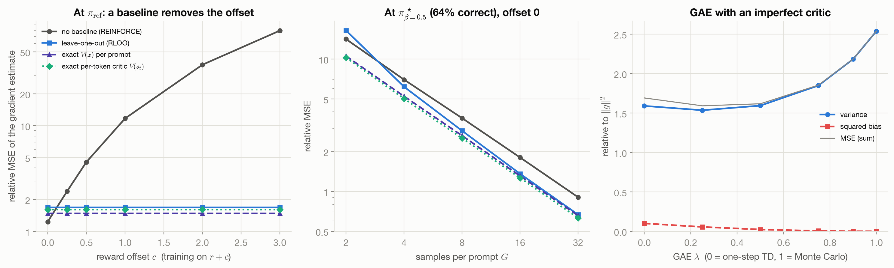
The left panel holds the policy at \(\pi_{\text{ref}}\) and adds a constant \(c\) to every reward. The expected gradient is identical for every \(c\). Without a baseline, the estimator’s error is about 1.2 times \(\|g\|^2\) at \(c=0\) and about 80 times at \(c=3\), growing with the square of the offset. Every baselined estimator is flat. This is the most important thing a baseline buys, and it matters more in LLM training than in the textbook setting: a reward model trained on preferences is identifiable only up to a per-prompt constant (the rewards chapter), so its offset is arbitrary. A baseline makes the gradient indifferent to it.
The same panel holds a surprise. At \(c = 0\), the estimator without a baseline has the lowest error of all. With a 0/1 reward and a policy that is usually wrong, most samples have reward 0 and contribute nothing; zero happens to be close to the average reward, so it is already a decent baseline. A baseline estimated from a few other samples adds its own noise, and here that costs more than it saves. Once the policy is better (middle panel, \(\pi^\star_{\beta=0.5}\), 64% correct on average and 85–95% on the two easiest prompts), the situation reverses: most rewards are now 1, zero is a poor baseline, and every baselined estimator beats plain REINFORCE from \(G = 4\) on. RLOO pays for estimating its baseline from only \(G-1\) samples: at \(G = 2\) its one-sample baseline is noisy enough to make it slightly worse than no baseline, and it has nearly caught up with the exact per-prompt value \(V(x)\) by \(G = 16\). The exact per-token critic \(V^\pi(s_t)\), the best a learned critic could be, is the best estimator at the better policy, but only slightly. In this task every prefix can still be completed correctly by the last token, so knowing the prefix says little about the outcome, and a per-token critic has little to add over a per-prompt baseline. The general lesson is that a baseline guarantees an unchanged expectation and invariance to the reward’s offset; how much it reduces variance depends on the reward and the policy, and should be measured rather than assumed.
Generalized advantage estimation
A critic opens a second design dimension. With a learned \(V_\phi\), the advantage of the token chosen at \(s_t\) can be estimated by the full Monte Carlo return minus the baseline, \(G_t - V_\phi(s_t)\), or by the one-step temporal-difference error \(\delta_t = r_{t+1} + \gamma V_\phi(s_{t+1}) - V_\phi(s_t)\), which bootstraps from the critic’s estimate of the next state. Schulman et al.’s generalized advantage estimator (GAE) interpolates with an exponentially weighted sum of TD errors (Schulman et al. 2015):
\[ \hat A_t^{\text{GAE}(\gamma,\lambda)} = \sum_{l=0}^{\infty}(\gamma\lambda)^l\,\delta_{t+l}, \qquad \delta_t = r_{t+1} + \gamma V_\phi(s_{t+1}) - V_\phi(s_t). \] \(\lambda = 1\) gives \(G_t - V_\phi(s_t)\); \(\lambda = 0\) gives \(\delta_t\).
The paper states the trade-off precisely. \(\lambda = 1\) is unbiased “regardless of the accuracy of \(V\), but it has high variance due to the sum of terms”; \(\lambda = 0\) is unbiased only if the critic is exact “and otherwise induces bias, but it typically has much lower variance” (Schulman et al. 2015, sec. 3). The right panel of Figure 2.2 measures it with a critic that equals the true value plus a fixed error of standard deviation 0.15 per state. Moving \(\lambda\) from 1 to 0 cuts the variance from about 2.5 to 1.6 (relative to \(\|g\|^2\)) and raises the squared bias from about 0.001 to 0.1; the total error is lowest at intermediate \(\lambda\). This is the bias–variance trade-off of bootstrapping from the previous chapter, now inside a policy-gradient estimator. GAE is what PPO-based RLHF uses (the shared-target chapter), and its dependence on a good critic is one reason later LLM recipes dropped the critic altogether.
GAE is built exactly like the λ-return of TD(λ), as its authors note, “however TD(λ) is an estimator of the value function, whereas here we are estimating the advantage function” (Schulman et al. 2015). The λ dial is the Monte Carlo vs. TD dial from every RL course.
2.6 Behavior and failure modes
No variation, no signal. With a baseline built from the same group, a prompt where every sampled response gets the same reward produces advantages of exactly zero, whether all the answers were right or all wrong. On the hard prompt of the previous chapter, most early groups were all wrong, and learning stalled until the policy happened onto correct answers. Policy Gradients Without a Critic quantifies how often this happens and what DAPO’s dynamic sampling does about it.
On-policy, strictly. The derivation required \(y\sim\pi_\theta\) for the current \(\theta\). The moment the policy is updated, last step’s samples come from the wrong distribution, and reusing them gives a biased gradient. Every practical method reuses samples somewhat, for efficiency, and needs a correction (importance ratios) and a guard against using it too far (a trust region). That is the next chapter.
The objective has no brakes. As noted under Interpretation, \(\mathbb{E}[r]\) rewards collapse onto whatever scores highest, and with a learned reward, onto whatever fools the reward model (the rewards chapter).
Credit is smeared across tokens. A single sequence-level weight multiplies every token’s score, so the tokens that mattered and the tokens that did not are pushed equally. On average the irrelevant pushes cancel; on any one sample they are noise. Per-token critics, process rewards and dense teacher signals (Learning by Imitating a Better Distribution) are all attempts to fix this.
2.7 Connections
- Keeping Updates Stable starts where the on-policy failure mode ends: importance ratios let a batch be reused, and clipping and KL terms stop the reuse from going wrong.
- The LLM as a Policy asks whether the right unit of action is a token or a whole response; the sequential derivation above shows that, with one terminal reward, the two views give the same gradient.
- The Shared Target, and RLHF with PPO assembles the pieces of this chapter (REINFORCE, a learned critic, GAE) into the PPO-based RLHF recipe.
- Policy Gradients Without a Critic revisits the baselines here (RLOO, the group mean, GRPO’s normalization) in the form LLM recipes actually use them, and shows what the normalization changes.