9 Learning by Imitating a Better Distribution
The policy gradient pushes up the log-probability of sampled responses with a signed weight. A second family of methods gets most of the benefit with less machinery: produce a better set of responses than the policy currently does, then do ordinary supervised learning on them. Best-of-\(n\) sampling, rejection-sampling fine-tuning, RAFT, STaR, ReST and expert iteration filter the policy’s own samples by a reward. Distillation, off- or on-policy, takes the better responses (or better next-token distributions) from a stronger model. Both halves of this chapter rest on one idea: supervised learning on samples from something better than the current policy. In the \((q,w)\) form that is \(w = 1\) on samples from a better \(q\), or \(w = \mathbb{1}[\text{good}]\) on samples from the current one. This chapter makes the idea precise: which “better distribution” each method imitates, when that is exactly the \(\pi^\star\) of the shared-target chapter, and what these methods give up for their robustness.
9.1 The problem
Improve a policy using a reward (or a teacher), without the variance, the trust region or the critic of policy-gradient RL. The constraint is self-imposed: every update must be a supervised maximum-likelihood step on some dataset.
9.2 Assumptions
- A way to judge or produce good responses: a reward to filter by, or a teacher to sample or score.
- Enough samples that some are good. Filtering throws away everything else, so a prompt the policy never answers well contributes nothing (the zero-signal problem of the critic-free chapter, in a sharper form).
- The policy can represent the better distribution, as in the idealized analysis of the shared-target chapter.
9.3 Filtered imitation
Why filtering is RL
STaR’s authors make the connection themselves. Treating the rationale as a latent variable and the reward as \(\mathbb{1}(\hat y = y)\), “STaR can be seen as an approximation to an RL-style policy gradient objective”: the log-derivative trick gives the gradient, and “the indicator function discards the gradient for all sampled rationales that do not lead to the correct answer: this is the filtering process in STaR” (Zelikman et al. 2022, sec. 3.1). The approximations, in their words, are greedy decoding (to reduce variance, at the cost of biased exploration) and “taking multiple gradient steps on the same batch of data (similar to some policy gradient algorithms)”.
In the book’s form, filtered imitation is REINFORCE with weight \(w = \mathbb{1}[\text{good}]\) on samples from the current (or an older) policy. Two things distinguish it from the policy gradient. The weight is never negative, so wrong samples carry no gradient: nothing pushes them down except normalization. And the dataset is used for many supervised steps, not one gradient step.
The family differs mostly in the filter and the schedule. RAFT samples, ranks with a reward model, keeps the best and fine-tunes on them, presented as an alternative to “the inefficiencies and instabilities associated with RL algorithms” (Dong et al. 2023). Yuan et al. named rejection-sampling fine-tuning (RFT) for collecting “correct reasoning paths as augmented fine-tuning datasets” for math (Yuan et al. 2023). ReST alternates a Grow step (sample from the policy) and an Improve step (filter with an increasing threshold, then fine-tune), and found plain behavior cloning on the filtered data the best of the losses it tried (Gulcehre et al. 2023). Expert iteration is the general pattern from game playing, where tree search acts as an expert whose improved policies a network learns to imitate and then improves on (Anthony et al. 2017); ReST’s authors relate their method to it explicitly.
Supervised learning on samples weighted by their reward is Peters and Schaal’s reward-weighted regression (Peters and Schaal 2007). Advantage-weighted regression derives the weights from a KL-constrained policy improvement step, whose optimum is \(\pi^\star(a\mid s) \propto \mu(a\mid s)\exp\big(\tfrac1\beta(R - V(s))\big)\) for a behavior policy \(\mu\), and then fits it by weighted maximum likelihood (Peng et al. 2019). With \(\mu = \pi_{\text{ref}}\) that is exactly this book’s \(\pi^\star\). Hard filtering is the limit of these weights as \(\beta\to0\).
Which distribution does filtering imitate?
The connection to the shared-target chapter can be made exact. Sample from \(\pi_{\text{ref}}\) and accept each sample with probability \(e^{(r - r_{\max})/\beta}\): the accepted samples are distributed exactly as \(\pi^\star = \pi_{\text{ref}}e^{r/\beta}/Z\). Supervised learning on them targets \(\pi^\star\). Equivalently, keep every sample but weight it by \(e^{r/\beta}\), which is reward-weighted regression with exponential weights; its population optimum is also \(\pi^\star\).
\[ y\sim\pi_{\text{ref}}(\cdot\mid x),\quad \text{accept with probability } e^{(r(x,y)-r_{\max})/\beta} \;\Longrightarrow\; y\sim\pi^\star(\cdot\mid x); \qquad \max_\theta\ \mathbb{E}_{y\sim\pi_{\text{ref}}}\big[e^{r(x,y)/\beta}\log\pi_\theta(y\mid x)\big] \text{ is maximized at } \pi^\star . \]
| Signal | scalar reward, used only to accept or reject |
| Samples from (\(q\)) | \(\pi_{\text{ref}}\) (one round; iterated variants resample from the current policy) |
| Per-sample weight (\(w\)) | 1 if accepted, 0 otherwise (or \(e^{r/\beta}\) for the weighted version) |
| Stability | none needed: it is supervised learning on a fixed dataset |
| Credit granularity | sequence level |
| Models in memory | policy (+ the reward to filter by) |
| Targets | \(\pi^\star\) exactly with acceptance \(e^{(r-r_{\max})/\beta}\); hard filters target something sharper |
| Classical lineage | rejection sampling + behavior cloning; reward-weighted regression |
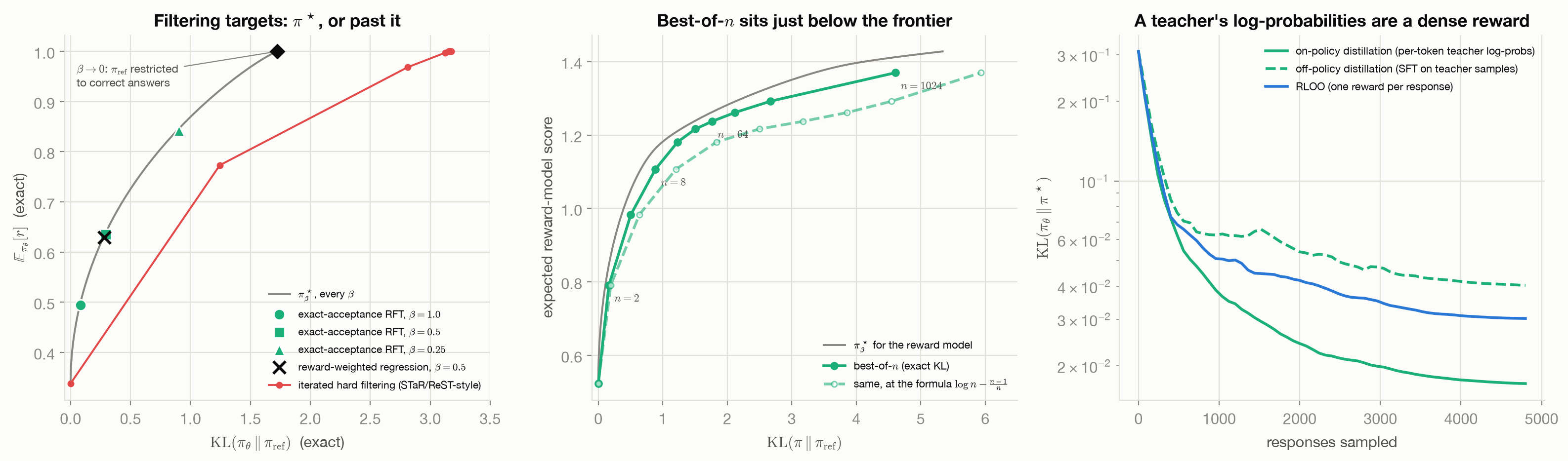
The left panel of Figure 9.1 checks this on the toy language. Exact-acceptance RFT at \(\beta = 1, 0.5, 0.25\) (100,000 proposals per prompt) lands on the frontier of \(\pi^\star_\beta\), at the point for its \(\beta\), and reward-weighted regression at \(\beta = 0.5\) lands on the same point as RFT. Practical recipes do not use exact acceptance. They keep the correct answers or the best of \(n\): hard filters. A hard filter on a 0/1 reward from \(\pi_{\text{ref}}\) samples targets the \(\beta\to0\) end of the frontier, \(\pi_{\text{ref}}\) restricted to correct answers (the diamond).
Iterated, hard filtering goes past even that. The red path is the STaR/ReST pattern: sample 64 responses per prompt from the current policy, keep the correct ones, fine-tune, repeat. After a few iterations every answer is correct, but the policy keeps moving: it ends at a KL of 3.2 from \(\pi_{\text{ref}}\), nearly twice that of \(\pi_{\text{ref}}\) restricted to correct answers (1.7). Each round trains on a finite sample of the previous round’s correct answers, so frequently sampled answers become more frequent, and the policy collapses within the set of correct answers. On the hardest prompt its entropy goes to zero, where \(\pi_{\text{ref}}\) restricted to correct answers has 3.5 nats. Nothing in the objective asks for diversity, and nothing in a hard filter holds the policy near \(\pi_{\text{ref}}\); the KL term that defines \(\pi^\star\) is simply absent.
Best-of-\(n\)
Best-of-\(n\) needs no training at all: sample \(n\) responses and return the one the reward model scores highest. It is the inference-time version of filtering, and the rewards chapter used it as one of Gao et al.’s two optimizers. The middle panel of Figure 9.1 compares it with the KL-regularized optimum for the same reward model. Its exact distribution, computed by enumeration, lies just below the frontier of \(\pi^\star_\beta\): nearly as much reward per unit of KL as the optimum. The panel also shows a correction. The formula \(\log n - \frac{n-1}{n}\), commonly used for the KL of best-of-\(n\) (and used by Gao et al.), is an upper bound, not the exact value, as Beirami et al. show (Beirami et al. 2025). On the toy language the exact KL at \(n = 64\) is 1.77 against the formula’s 3.18; at \(n = 8\), 0.89 against 1.20. Plotted at the formula’s KL (dashed), best-of-\(n\) looks less efficient than it is.
What filtering gives up
Negative samples carry no gradient. A wrong answer that is filtered out teaches the model nothing directly. A policy gradient pushes it down; filtering only stops pushing it up. This is part of why filtering is so stable, and part of why it is slow when most samples are wrong.
The improvement per round is bounded by the filter. One round of filtering from a fixed policy can move at most as far as the best-of-\(n\) (or accepted) distribution, which is why recipes iterate, and iteration without a KL anchor brings the collapse in the left panel.
Robustness is the payoff. Supervised learning on a fixed dataset has no importance ratios, no clipping, no critic and no feedback loop within a round. When the filter is reliable (a verifier), this is a strong practical reason to prefer it, and it is why rejection sampling appears inside recipes that also use RL: DeepSeek-R1 uses rejection sampling from its RL checkpoint to build the SFT data for its next stage (DeepSeek-AI 2025).
9.4 Distillation, off- and on-policy
The second way to get a better distribution is to have one: a stronger teacher model.
Off-policy distillation is SFT on the teacher’s outputs, sequence-level knowledge distillation in Kim and Rush’s term (Kim and Rush 2016). In the book’s form, \(q\) is the teacher and \(w = 1\), and it minimizes the forward KL from the teacher to the student, which is mass-covering (keeping updates stable). Its weakness is the one every chapter of Part II has met: the student is trained on the teacher’s states, not its own, so its own mistakes take it to states the training never covered.
On-policy distillation fixes that the way DAgger does. Agarwal et al.’s generalized knowledge distillation (GKD) trains the student on a mixture of fixed data and its own samples, with the teacher providing the target distribution at every token, and a choice of divergence (forward KL, reverse KL, or a generalized Jensen–Shannon divergence); they frame the problem as imitation learning with train–inference mismatch and note that it “can be easily combined with RL fine-tuning” (Agarwal et al. 2023). Thinking Machines’ recipe makes the RL view explicit: the student samples, the teacher scores every token, and “we set the per-token advantage to the negative reverse KL”, with “a discount factor of zero” (Lu and Thinking Machines Lab 2025). The teacher’s log-probability is then a dense reward: every token gets its own signal, exactly where the student departs from the teacher, instead of one number per response. The authors frame the difference in information terms, \(O(N)\) bits per episode for \(N\) tokens against roughly one for a sequence-level reward, and report large compute savings relative to RL on their tasks (Lu and Thinking Machines Lab 2025) (a lab’s own report).
| Signal | the teacher’s per-token log-probabilities |
| Samples from (\(q\)) | the student \(\pi_\theta\) itself (on-policy) |
| Per-sample weight (\(w\)) | per token: \(-(\log\pi_\theta(y_t\mid s_t) - \log\pi_T(y_t\mid s_t))\), the negative per-token reverse KL, with no discounting |
| Stability | none needed beyond a small learning rate: the signal is dense and bounded by the teacher |
| Credit granularity | token level |
| Models in memory | student, teacher |
| Targets | the teacher’s distribution, by reverse KL (mode-seeking) |
| Classical lineage | DAgger (the expert labels the states the learner visits); a policy gradient with a dense, shaped reward |
The right panel of Figure 9.1 compares the three ways of reaching the same \(\pi^\star\) on the toy language, with the teacher set to \(\pi^\star\) itself. Per sampled response, on-policy distillation learns fastest, reaching about 0.017 nats after 4,800 sampled responses against about 0.03 for RLOO and 0.04 for off-policy distillation. The advantage is about a factor of two here. A four-token response leaves little room for per-token signal to help, and varying the response length from two to six tokens did not make the gap grow in this toy, so the toy can confirm the direction of the effect but not the large factors reported for long reasoning traces.
On the map of this book, on-policy distillation is the on-policy, dense-reward corner: RL’s data regime with supervised learning’s per-token signal. It is also the clearest case of the shared-target chapter’s theme: if the teacher is (close to) \(\pi^\star\), then distillation is one more route to \(\pi^\star\), and in the signature figure it was the closest of the sampled methods.
9.5 Connections
- Policy Gradients supplies the gradient that filtering approximates; the difference is the weight, never negative here.
- The Shared Target, and RLHF with PPO supplies the distribution that exact-acceptance filtering and reward-weighted regression target, and the signature figure in which on-policy distillation was the closest sampled route to it.
- What RL Actually Does to a Model returns to the collapse of iterated filtering: losing diversity while improving reward is one of the central findings about RL-trained models.
- Rewarding Calibration changes the signal instead of the sampler: a reward that scores stated confidence, which hard filtering on correctness cannot express.