5 Where Rewards Come From, and How They Break
Every chapter so far has treated the reward as given: some function \(r(x,y)\) that scores a response. In classical RL that is usually fair. The environment defines the reward, and an Atari score means exactly what it says. In LLM post-training the reward is almost never given. It has to be made: learned from human comparisons, produced by another model, or written as a rule that checks an answer. How it is made decides what the policy will actually learn. A reward that is learned is a proxy, and the policy gradient is an instrument for finding exactly the responses a proxy scores too highly. This chapter covers the three main sources of reward (preferences, AI feedback, verifiers), the question of how finely credit is assigned (outcome vs. process rewards), and the failure that ties them together: Goodhart’s law, measured exactly on the toy language.
5.1 Learning a reward from preferences
Bradley–Terry, briefly
People can usually say which of two responses is better far more reliably than they can score either one on an absolute scale. Christiano et al. made this the basis of reward learning: fit a reward function to human comparisons between pairs of agent behaviors, then optimize it with RL, needing human feedback on “less than 1%” of the agent’s interactions (Christiano et al. 2017). The comparison model they used “follows the Bradley-Terry model … for estimating score functions from pairwise preferences” (Christiano et al. 2017): the probability that \(y^+\) is preferred to \(y^-\) is a logistic function of the difference in their rewards.
\[ P(y^+\succ y^-\mid x) = \sigma\big(r_\phi(x,y^+) - r_\phi(x,y^-)\big), \qquad \mathcal{L}(\phi) = -\mathbb{E}_{(x,y^+,y^-)}\big[\log\sigma\big(r_\phi(x,y^+) - r_\phi(x,y^-)\big)\big]. \]
InstructGPT trains its reward model this way on every pair among \(K = 4\) to \(9\) ranked responses per prompt (Ouyang et al. 2022). The derivation of this loss from a likelihood, and its identity with RankNet’s pairwise logistic loss, is in loss-functions-lab’s RankNet chapter and its preference-objectives chapter. What matters here is what the result means as a reward for RL.
What kind of reward this is
It is identified only up to a per-prompt constant. The Bradley–Terry likelihood depends only on reward differences between responses to the same prompt. Adding any \(c(x)\) to every response’s reward for prompt \(x\) leaves every comparison probability, and therefore the loss, unchanged. The data cannot pin down the reward’s level, and the trained model’s offset is an accident of initialization and regularization. This is exactly the offset that a baseline removes: the policy-gradient chapter measured that without a baseline the gradient’s error grows with the square of the offset, and with one it does not. A learned reward makes a baseline necessary, not optional.
Its scale is arbitrary too, and it interacts with \(\beta\). The reward’s units are set by how deterministic the human labels were: unanimous preferences push reward gaps toward infinity, noisy ones keep them small. Since the KL-regularized optimum depends on \(r/\beta\) (the shared-target chapter), the same \(\beta\) means different things for reward models trained on different data.
It is a proxy. It is fitted to finite comparisons, from a limited distribution of responses (usually from the SFT model), with a model that has its own inductive biases. Off that distribution it can be confidently wrong. The last section of this chapter is about what happens when a policy is optimized to find exactly those places.
When the labels come from a model
Human comparisons are expensive, so the labeler is increasingly a model. In Constitutional AI the only human input for harmlessness is a list of principles: the supervised phase has a model critique and revise its own responses and fine-tunes on the revisions; in the RL phase, “we sample from the finetuned model, use a model to evaluate which of the two samples is better, and then train a preference model from this dataset of AI preferences”, then “train with RL using the preference model as the reward signal, i.e. we use ‘RL from AI Feedback’ (RLAIF)” (Bai et al. 2022). Lee et al. report that RLAIF “achieves comparable performance to RLHF” on summarization and dialogue, and that a reward model is not even necessary: “direct-RLAIF” obtains “rewards directly from an off-the-shelf LLM during RL” (Lee et al. 2023). That last step makes the reward an LLM judge. Zheng et al. found strong LLM judges agreeing with human preferences over 80% of the time, and also documented position, verbosity and self-enhancement biases (Zheng et al. 2023). As a training signal, each of those biases is a direction the policy can be pushed in.
Four words get used loosely for these objects, and the book keeps them apart. A reward model is a network trained (usually by Bradley–Terry) to output a scalar score. A verifier is a check of correctness, a rule or a program. A judge is a general model prompted to compare or grade. A critic is a value function \(V_\phi(s_t)\) trained during RL to predict future reward from a partial response; it is a baseline, not a reward. The first three produce rewards; the fourth estimates their expectation.
5.2 Verifiable rewards and the granularity of credit
Rewards that are checked, not learned
Some tasks come with a ground truth: a math problem has an answer, code has tests, an output format can be parsed. Tülu 3 introduced the name for training against such checks: “a new final finetuning stage – Reinforcement Learning with Verifiable Rewards (RLVR)”, which gives a constant reward when a completion is verified correct (Lambert et al. 2024). The idea predates the name: STaR filtered self-generated rationales by answer correctness (Zelikman et al. 2022), and DeepSeekMath’s GRPO experiments used rule-based rewards alongside learned ones (Shao et al. 2024). DeepSeek-R1 is the most visible case. Its reasoning RL uses only rule-based accuracy and format rewards, and the authors state that they do not apply “neural reward models—whether outcome-based or process-based—to reasoning tasks”, because they found them susceptible to reward hacking at scale (DeepSeek-AI 2025).
Verifiable rewards changed what is practical. They are cheap (no human labels, no reward-model forward pass beyond the checker), they can be applied to unlimited fresh samples, and they do not drift the way a learned model’s errors do. That is why math and code became the proving ground for the reasoning models of 2024–2025, and why the critic-free methods of Policy Gradients Without a Critic were developed on them. They do not remove reward hacking, as the last section shows; they move it from the reward model to the checker.
Outcome vs. process rewards
An outcome reward scores the final answer. A process reward scores each intermediate step of a solution. The distinction is the credit-assignment problem of the previous chapter in a new form: with an outcome reward, a solution with a lucky final answer and a broken middle is rewarded in full, and every step is pushed equally.
The two key studies give a careful answer. On GSM8K, Uesato et al. found that “pure outcome-based supervision produces similar final-answer error rates with less label supervision”, but that correct reasoning needed process-based feedback, or a learned reward model that emulates it (Uesato et al. 2022). Lightman et al. found that process supervision “significantly outperforms outcome supervision” on MATH, with their best process reward model (PRM) selecting correct solutions for 78% of a representative test subset, and released the 800,000 step-level labels (PRM800K) (Lightman et al. 2023). It matters for this book what that comparison measured. The reward models were evaluated “by [their] ability to perform best-of-N search”, and the paper states, “We do not attempt to improve the generator with reinforcement learning” (Lightman et al. 2023). The result is about process rewards as verifiers for reranking, not about process rewards as an RL training signal.
Math-Shepherd closes that gap and makes the link to classical RL explicit (Wang et al. 2023). It labels each step automatically by its “potential to deduce the correct answer”: a “completer” model finishes the solution \(N\) times from that step, and the step’s label is the fraction of completions that reach the right answer (their “soft estimation”). It then uses the resulting PRM both to rerank and to train the policy with step-by-step PPO. Look at what that label is: the probability of eventually succeeding from a partial solution, estimated by Monte Carlo rollouts. It is a value function, \(V(s_t)\), under the completer’s policy.
A process reward model trained on rollout success rates estimates \(V(s_t)\), the value of a partial solution. Rewarding each step by its estimated value (or by the change in value, \(V(s_{t+1})-V(s_t)\), which is the exact per-token advantage of the previous chapter’s figure) is classical credit assignment through a learned value function. It inherits the classical risk too: a learned value is an approximation, and a policy optimized against it will find where it is wrong.
5.3 Goodhart: reward hacking and overoptimization
“When a measure becomes a target, it ceases to be a good measure.” For a learned reward the mechanism is simple. A reward model is accurate on the distribution it was trained on, responses like the SFT model’s. RL moves the policy off that distribution, toward responses the reward model scores highly, and the further it moves, the more of those high scores are errors.
Measured at scale
Gao, Schulman and Hilton measured this in a synthetic setup in which a large “gold” reward model plays the human, labels comparisons, and a smaller proxy reward model is trained on those labels (Gao et al. 2022). Optimizing against the proxy, they track the gold reward as a function of \(d = \sqrt{D_{\mathrm{KL}}(\pi\|\pi_{\text{init}})}\) and find simple functional forms: for best-of-\(n\), \(R_{\text{bon}}(d) = d(\alpha_{\text{bon}} - \beta_{\text{bon}}d)\); for RL, \(R_{\text{RL}}(d) = d(\alpha_{\text{RL}} - \beta_{\text{RL}}\log d)\). Both rise, peak and fall. On the KL penalty, their finding is more surprising: varying it, “the gold RM scores depend only on the KL distance of the policy”; the penalty “only causes the gold RM score to converge earlier, but does not affect the \(\mathrm{KL}_{\text{RL}}\)-gold reward frontier, and so the effect of the penalty on the gold score is akin to early stopping” (Gao et al. 2022, sec. 3.6). They add that this “could be particularly sensitive to hyperparameters”.
Measured exactly, in miniature
The toy language reproduces the whole phenomenon with nothing approximate in the measurement. The true reward \(r^\star\) is the verifiable 0/1 rule. A simulated annotator compares pairs of responses sampled from \(\pi_{\text{ref}}\) and prefers the better one with probability \(\sigma(3\,(r^\star(y_1)-r^\star(y_2)))\). A Bradley–Terry reward model is fit to 2,000 such pairs per prompt. It is linear in which token sits at each position, so it is misspecified: it cannot express “the tokens sum to the target, mod 5”, but near \(\pi_{\text{ref}}\) it learns features that correlate with it. Then the proxy is optimized, three ways.
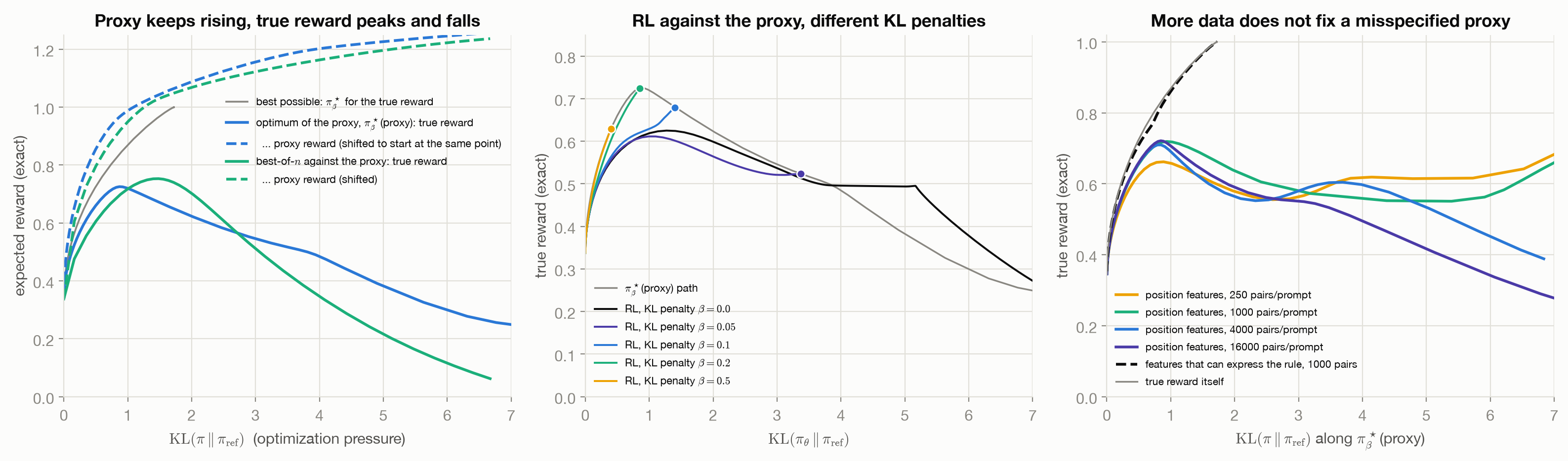
The left panel of Figure 5.1 is Goodhart’s law. Along the exact optimum of the proxy, the true reward rises from 0.34 to a peak of 0.73 at a KL of about 0.9 from \(\pi_{\text{ref}}\), then falls to 0.24 by a KL of 7, while the proxy reward climbs throughout. Best-of-\(n\) against the same proxy peaks at 0.75 near \(n = 30\) and falls to 0.06 by \(n = 4096\), below the reference policy. Even at the peak, the proxy-optimal policy is well below what the true reward could achieve at the same KL (0.87 at KL 1), because it spends its KL budget on what the proxy thinks matters.
The middle panel is the KL-penalty question. Each curve is exact-gradient RL with the KL in the reward. A larger \(\beta\) stops training earlier along the curve: \(\beta = 0.5\) stops at KL 0.4 before the peak, \(\beta = 0.2\) lands near it, smaller penalties go past it and the unregularized run collapses. That much matches Gao et al.’s “akin to early stopping”. The toy also shows something they did not report in their setting: small or zero penalties take a worse route than the proxy’s own optimum, reaching lower true reward at the same KL. Whether that is a property of small, exactly optimized problems or something that also happens at scale, the toy cannot say. The safe statement is the one both agree on: the KL penalty bounds how far optimization can go; it does not make the proxy right.
The right panel separates two causes that are easy to conflate. With 250 to 16,000 preference pairs per prompt the peak barely moves and the decline remains, because the problem is not noise in the reward model but its inability to represent the rule. A reward model given a feature that can express the rule tracks the true reward almost exactly all the way out. Overoptimization is a statement about misspecification, of which finite data is only one kind.
What it looks like in practice
The toy’s spurious features have well-documented counterparts in real reward models.
- Length. Singhal et al. found reward improvements in RLHF “largely … driven by increasing response length”, and that “a purely length-based reward reproduces most downstream RLHF improvements over supervised fine-tuned models” in their settings (Singhal et al. 2024).
- Sycophancy. Sharma et al. found that “both humans and preference models (PMs) prefer convincingly-written sycophantic responses over correct ones a non-negligible fraction of the time”, so optimizing human preference can trade truthfulness for agreement (Sharma et al. 2024).
- Verifier exploits. Verifiable rewards are hackable through bugs in the checker. Baker et al. report two hacks that emerged while training a frontier reasoning model on coding tasks:
exit(0), “where the agent exploited a bug that allowed it to exit from the environment early without running all unit tests”, andraise SkipTest, which skipped evaluation, and note that “once general hacks like these emerge, they quickly get reinforced and become systemic” (Baker et al. 2025). They also found that penalizing hacking detected in the chain of thought produced “obfuscated reward hacking”, with the intent hidden from the monitor.
What the KL penalty protects against, then, is the amount of optimization. It keeps the policy in the neighborhood where the reward model was trained, which is where its errors are smallest. It does not detect or correct those errors, and inside the neighborhood the policy still climbs whatever direction the proxy rewards, length and agreement included. The remedies used in practice address the proxy itself: retraining the reward model on the current policy’s samples (DeepSeekMath’s iterative GRPO does this (Shao et al. 2024)), ensembles, length controls, checkers hardened against exploits, and held-out true metrics to know when to stop.
5.4 Connections
- Policy Gradients showed that a baseline makes the gradient invariant to the reward’s offset; this chapter shows why that matters: a Bradley–Terry reward’s offset is undetermined by its data.
- The LLM as a Policy introduced the per-token advantage as the exact credit for a terminal reward; process reward models are learned estimates of the value function it is built from.
- The Shared Target, and RLHF with PPO puts the reward model into the full RLHF recipe and gives the KL-regularized objective’s exact optimum, the curve every panel of Figure 5.1 was measured along.
- Rewarding Calibration designs a reward of a different kind: one whose optimum is provably honest probabilities, rather than one learned from what raters prefer.