7 Direct Preference Methods
RLHF with PPO reaches the KL-regularized optimum \(\pi^\star\) the expensive way: train a reward model, then run on-policy RL against it with four networks in memory and generation inside the loop. The shared-target chapter ended with a formula that suggests a shortcut. If the optimal policy is the reference tilted by \(\exp(r/\beta)\), then the reward can be read back off the optimal policy. Direct Preference Optimization takes that literally: it writes the reward as a function of the policy, substitutes it into the Bradley–Terry likelihood of the preference data, and fits the policy to the comparisons directly, by logistic regression, with no reward model and no sampling. This chapter derives DPO from the RL side, measures on the toy language what the shortcut gives up by going offline, and then reads the main variants (IPO, KTO, SimPO, ORPO) as answers to one question each: which assumption did the method change?
7.1 The problem
Given a dataset of comparisons \((x, y^+, y^-)\) and a reference policy, find the policy that RLHF would have found, the optimum of \(\mathbb{E}_{\pi}[r] - \beta D_{\mathrm{KL}}(\pi\|\pi_{\text{ref}})\) for the Bradley–Terry reward behind the comparisons, without ever fitting that reward explicitly and without sampling from the policy.
7.2 Assumptions
- Preferences follow Bradley–Terry with some reward \(r\): \(P(y^+\succ y^-\mid x) = \sigma(r(x,y^+) - r(x,y^-))\).
- The goal is the KL-regularized optimum for that reward, \(\pi^\star\propto\pi_{\text{ref}}\exp(r/\beta)\).
- The policy class can represent \(\pi^\star\), as in the idealized analysis of the shared-target chapter.
7.3 Derivation
Invert the closed form for any prompt \(x\): \(r(x,y) = \beta\log\frac{\pi^\star(y\mid x)}{\pi_{\text{ref}}(y\mid x)} + \beta\log Z(x)\). The partition function is intractable, but Bradley–Terry only ever needs reward differences between two responses to the same prompt, and \(\beta\log Z(x)\) cancels in every difference. Replacing \(\pi^\star\) by the policy being trained, \(\pi_\theta\), defines an implicit reward \(\hat r_\theta(x,y) = \beta\log\frac{\pi_\theta(y\mid x)}{\pi_{\text{ref}}(y\mid x)}\), and the negative log-likelihood of the comparisons under Bradley–Terry with this reward is the DPO loss (Rafailov et al. 2023):
\[ \mathcal{L}_{\text{DPO}}(\theta) = -\,\mathbb{E}_{(x,y^+,y^-)\sim\mathcal{D}}\Big[\log\sigma\Big(\beta\log\frac{\pi_\theta(y^+\mid x)}{\pi_{\text{ref}}(y^+\mid x)} - \beta\log\frac{\pi_\theta(y^-\mid x)}{\pi_{\text{ref}}(y^-\mid x)}\Big)\Big]. \]
The algebra of each step, and the identity of this loss with RankNet’s pairwise logistic loss, is derived in full in loss-functions-lab’s preference-objectives chapter; this book takes the RL view. Rafailov et al. show that the reparameterization loses nothing: “all reward classes consistent with the Plackett-Luce (and Bradley-Terry in particular) models can be represented with the reparameterization \(r(x,y) = \beta\log\frac{\pi(y\mid x)}{\pi_{\text{ref}}(y\mid x)}\)” (their Theorem 1), which is the precise sense of the paper’s subtitle, “your language model is secretly a reward model” (Rafailov et al. 2023).
The gradient, in the \((q,w)\) form
Differentiating gives (Rafailov et al. 2023)
\[ \nabla_\theta\mathcal{L}_{\text{DPO}} = -\beta\,\mathbb{E}_{\mathcal{D}}\Big[\sigma\big(\hat r_\theta(x,y^-) - \hat r_\theta(x,y^+)\big)\big(\nabla_\theta\log\pi_\theta(y^+\mid x) - \nabla_\theta\log\pi_\theta(y^-\mid x)\big)\Big]. \]
In this book’s form: the sampling distribution \(q\) is the fixed dataset, and the weight is \(+\beta\sigma(\hat r^- - \hat r^+)\) on the preferred response and the same with a minus sign on the rejected one. The weight is large exactly when the implicit reward orders the pair the wrong way; the authors write that “the examples are weighed by how much higher the implicit reward model \(\hat r_\theta\) rates the dispreferred completions”, with “higher weight when reward estimate is wrong” (Rafailov et al. 2023). A pair the policy already orders confidently contributes almost nothing.
| Signal | pairwise preferences \(y^+\succ y^-\) |
| Samples from (\(q\)) | a fixed dataset of pairs (offline) |
| Per-sample weight (\(w\)) | \(\pm\beta\,\sigma(\hat r_\theta^- - \hat r_\theta^+)\) on the preferred / rejected response |
| Stability | the log-ratio to \(\pi_{\text{ref}}\) inside the loss; no sampling, no clip |
| Credit granularity | sequence level |
| Models in memory | policy, reference (its log-probs can be precomputed) |
| Targets | \(\pi^\star\) exactly, for infinite data with full-support pairs; the optimum of the empirical loss otherwise |
| Classical lineage | none in RL: logistic regression (Bradley–Terry MLE) on an implicit reward; it targets an RL optimum without doing RL |
7.4 Interpretation: the same target, without RL
The test suite confirms the claim exactly. Minimizing the population DPO loss on the toy language, with pairs drawn from \(\pi_{\text{ref}}\) and labelled by Bradley–Terry from the true reward, recovers \(\pi^\star\) to within \(10^{-6}\) nats; so does drawing the pairs from a quite different distribution, as long as every response can appear (tests/test_dpo.py). That is the “DPO, infinite pairs” curve of the shared-target chapter’s signature figure, the fastest route to \(\pi^\star\) of all. With enough data, DPO and PPO-based RLHF aim at the same distribution.
DPO is therefore not RL in the sense of sampling and rewarding: nothing is sampled from the policy during training and no reward is evaluated. It is RL in the sense of its target. Which of the two senses matters depends on the question, and most of the rest of this chapter is about the cost of the first.
7.5 What going offline costs
Three costs follow from training on a fixed dataset, and each can be seen on the toy language.
No exploration. The gradient touches only responses in the dataset. A better response that neither the reference nor the annotators ever produced cannot be learned about. Its probability can still change, through normalization and shared parameters, but nothing pushes it up because it is good.
Distribution mismatch. The comparisons come from whatever policy generated them, usually not the current \(\pi_\theta\), and the further the policy moves, the less the data says about the responses it now produces. Rafailov et al. note the related problem that \(\pi_{\text{ref}}\) should be the policy that generated the data; when it is not available, they initialize the reference by “maximizing likelihood of preferred completions” to reduce the shift (Rafailov et al. 2023).
Overfitting the dataset. With finite data, many responses appear only as winners or only as losers, so the empirical preference is deterministic. The Bradley–Terry likelihood of a deterministic preference is maximized only by an infinite reward gap, which DPO reaches by driving log-ratios without bound, and the KL term inside the loss cannot stop it. Azar et al. make this argument formally: with deterministic or near-deterministic preferences, the reward difference must go to infinity, so the KL regularization becomes ineffective, whereas RLHF is protected in practice by its reward model’s underfitting (Azar et al. 2023). The left panel of Figure 7.1 shows it on the toy language. Offline DPO on 5,000 pairs per prompt approaches \(\pi^\star\) for about 50 steps and then moves away, ending at 0.19 nats after 800 steps. More data delays and shrinks the drift (20,000 pairs end near 0.05, 100,000 near 0.02). The same drift appears in The Shared Target, which trains for 1,000 steps with a different learning-rate schedule and reports the median of three seeds; there the 5,000-pair run ends further away, at 0.29 nats.
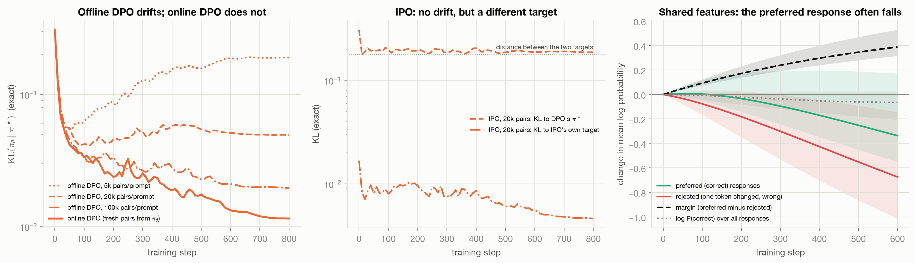
Likelihood displacement. DPO only asks for \(\hat r_\theta(y^+) > \hat r_\theta(y^-)\), a statement about a difference. Nothing requires the preferred response to become more likely, and in practice its probability often falls. Razin et al. study this in depth: the preferred response’s likelihood “often decreases during training”, the probability mass can move to responses with the opposite meaning, and in a safety setting the effect reduced one model’s refusal rate from 74.4% to 33.4%; they trace it to preferred and rejected responses with similar internal representations, measured by a “centered hidden embedding similarity” (CHES) score (Razin et al. 2025).
The toy language shows both why this can happen and why it needs shared structure. With the fully tabular policy, the preferred responses of informative pairs (correct over incorrect) become more likely during DPO; their mean log-probability rose from \(-1.78\) to \(-1.13\) in the 5,000-pair run behind the left panel. The average over all chosen responses falls (from \(-2.17\) to \(-2.37\)), but only because 69% of the pairs are between two equally good responses, where the “chosen” one won a coin flip and is often wrong. (That is a real hazard of noisy labels, but a different one.) The right panel uses a log-linear policy instead, in which a response’s score is a sum of per-position token weights, so responses that share tokens share parameters. It is trained with DPO on 100 pairs per prompt whose rejected response differs from the preferred one in a single token, for ten different random pair sets. In every run the rejected responses fall (median \(-0.67\)) and the margin grows (median \(+0.39\)), as intended. In six of the ten runs the preferred responses fall too (median change \(-0.34\) across all ten), and the overall probability of a correct answer slightly decreases (median \(-0.07\) in log-probability), even though every training pair prefers a correct answer: pushing down a rejected response’s tokens also pushes down the tokens it shares with the preferred one. Whether it happens in a given run depends on which pairs were drawn, which is consistent with Razin et al.’s finding that it is driven by the similarity structure of particular preference pairs. This is their mechanism, in miniature.
7.6 Online and iterative DPO
The fix for the offline costs is to stop being offline. Guo et al. observe that “preference datasets used in DAP [direct alignment from preferences] methods are usually collected ahead of training and never updated”, and propose online AI feedback: at each step, sample two responses “from the current model” and have an LLM annotator choose between them (Guo et al. 2024). Xiong et al. derive an iterative version of DPO from a reverse-KL-regularized contextual bandit formulation and report that it beats offline DPO (Xiong et al. 2023), and Noukhovitch et al. found online DPO the most robust to the staleness of asynchronous training (Noukhovitch et al. 2025).
The left panel of Figure 7.1 includes the online version: each step draws fresh pairs from the current policy and labels them by the same Bradley–Terry annotator. It keeps converging toward \(\pi^\star\) (about 0.01 nats after 800 steps), because there is no fixed dataset to overfit, and because the population DPO loss has the same minimizer for any full-support pair distribution, including the policy’s own. Online DPO is DPO’s loss with RL’s data regime. On the map of this book it sits next to the on-policy methods, and it shows that the distinction between “RL” and “preference optimization” is mostly a distinction between data regimes.
Offline DPO has the weakness of every method trained on a fixed dataset of someone else’s behavior: the learner’s own outputs drift to where the data says nothing. Collecting fresh comparisons on the current policy’s samples is the remedy imitation learning found in DAgger and RL found in on-policy sampling, applied to a logistic-regression loss.
7.7 The variants, as changed assumptions
Dozens of DPO variants exist. Four illustrate distinct axes; for each, the question is which of DPO’s assumptions it changes and what that buys and costs.
IPO: bound the preference transform
Azar et al. place RLHF and DPO in a family, ΨPO, that maximizes \(\mathbb{E}[\Psi(p^\star(y\succ y'\mid x))] - \tau D_{\mathrm{KL}}(\pi\|\pi_{\text{ref}})\) for some function \(\Psi\) of the preference probability (Azar et al. 2023). Bradley–Terry with a reward corresponds to an unbounded \(\Psi\) (the logit), which is why deterministic preferences push the reward gap to infinity. IPO takes \(\Psi\) to be the identity, and its empirical loss becomes a squared regression of the log-ratio gap \(h_\theta(y^+,y^-) = \log\frac{\pi_\theta(y^+)\pi_{\text{ref}}(y^-)}{\pi_\theta(y^-)\pi_{\text{ref}}(y^+)}\) onto a fixed target, \(\mathbb{E}\big[(h_\theta - \tfrac{1}{2\tau})^2\big]\) (Azar et al. 2023). A bounded target cannot be overfitted to infinity.
The changed assumption also changes the target. With \(\Psi\) the identity, the optimum tilts \(\pi_{\text{ref}}\) by the probability of winning a comparison against the data distribution, \(\pi^{\text{IPO}}\propto\pi_{\text{ref}}\exp\big(p(y\succ\mu)/\tau\big)\), not by the reward. The middle panel of Figure 7.1 computes that optimum exactly: IPO on 20,000 pairs per prompt converges to it (within 0.005 nats) with no drift. That optimum is 0.18 nats from DPO’s \(\pi^\star\) (the trained IPO policy ends 0.19 nats away), a distribution with noticeably lower expected reward on the toy task. IPO trades the reward-based target for robustness.
| Signal | pairwise preferences |
| Samples from (\(q\)) | a fixed dataset of pairs (offline) |
| Per-sample weight (\(w\)) | \(\pm 2(\tfrac{1}{2\tau} - h_\theta)\): a regression residual, bounded and signed |
| Stability | KL to \(\pi_{\text{ref}}\) via the bounded target \(\tfrac{1}{2\tau}\) |
| Credit granularity | sequence level |
| Models in memory | policy, reference |
| Targets | \(\pi_{\text{ref}}\) tilted by the preference probability \(p(y\succ\mu)/\tau\), not by a reward |
| Classical lineage | none in RL: least-squares regression of a log-ratio gap |
KTO: unpaired, binary feedback
Pairs are expensive; a thumbs-up or thumbs-down on a single response is cheap. KTO needs only “a binary signal of whether an output is desirable or undesirable for an input” (Ethayarajh et al. 2024). It keeps DPO’s implicit reward \(r_\theta = \log\frac{\pi_\theta}{\pi_{\text{ref}}}\) but scores each response against a reference point \(z_0\) rather than against a paired alternative: desirable responses earn \(c_D\,\sigma(\beta(r_\theta - z_0))\) and undesirable ones \(c_U\,\sigma(\beta(z_0 - r_\theta))\) (the paper’s \(\lambda_D\) and \(\lambda_U\)). The reference point is a batch estimate of the KL between policy and reference, “biased but convenient”, and the authors “do not backpropagate through \(z_0\)” (Ethayarajh et al. 2024). The framing is Kahneman and Tversky’s prospect theory: value is measured relative to a reference point, with possibly different weights for gains and losses. The changed assumption is the data model: unpaired binary labels instead of Bradley–Terry pairs.
| Signal | binary desirable / undesirable labels on single responses (no pairs) |
| Samples from (\(q\)) | a fixed dataset of labelled responses (offline) |
| Per-sample weight (\(w\)) | \(\pm c_{D/U}\,\beta\,\sigma'(\cdot)\): the slope of a sigmoid of \(r_\theta - z_0\), signed by the label |
| Stability | the log-ratio to \(\pi_{\text{ref}}\); the batch reference point \(z_0\) |
| Credit granularity | sequence level |
| Models in memory | policy, reference |
| Targets | a prospect-theoretic utility of the implicit reward, not exactly \(\pi^\star\) |
| Classical lineage | none in RL; behavioral economics (prospect theory) |
SimPO: drop the reference, normalize by length
SimPO replaces the implicit reward with the average log-probability per token, \(\frac{\beta}{|y|}\log\pi_\theta(y\mid x)\), and adds a target margin \(m\) (the paper’s \(\gamma\)): \(-\log\sigma\big(\frac{\beta}{|y^+|}\log\pi_\theta(y^+) - \frac{\beta}{|y^-|}\log\pi_\theta(y^-) - m\big)\) (Meng et al. 2024). Two assumptions change. There is no reference model, which saves its memory and compute but removes the anchor that defines \(\pi^\star\): SimPO no longer targets the KL-regularized optimum of anything. And the reward is length-normalized, motivated by the observation that DPO’s implicit reward and the average log-likelihood that drives generation disagree on many pairs, and by length bias (Meng et al. 2024).
| Signal | pairwise preferences |
| Samples from (\(q\)) | a fixed dataset of pairs (offline) |
| Per-sample weight (\(w\)) | \(\pm\frac{\beta}{|y|}\sigma(-\text{margin})\), per response, with the length normalization inside |
| Stability | the target margin \(m\); no reference, no KL |
| Credit granularity | sequence level, length-normalized |
| Models in memory | policy only |
| Targets | does not target \(\pi^\star\): without \(\pi_{\text{ref}}\) there is no KL-regularized objective |
| Classical lineage | none in RL: a margin-based logistic loss on average log-likelihoods |
ORPO: fold the preference into SFT
ORPO removes the reference model and the separate SFT stage. Its loss is the SFT negative log-likelihood of the preferred response plus \(c_{\text{OR}}\) (the paper’s \(\lambda\)) times an odds-ratio term, \(\mathcal{L}_{\text{SFT}} + c_{\text{OR}}\mathcal{L}_{\text{OR}}\) with \(\mathcal{L}_{\text{OR}} = -\log\sigma\big(\log\frac{\text{odds}_\theta(y^+\mid x)}{\text{odds}_\theta(y^-\mid x)}\big)\) and \(\text{odds}(y) = P(y)/(1 - P(y))\) for the length-normalized (geometric-mean) probability (Hong et al. 2024). The changed assumption is the pipeline: preference alignment happens “without a reference model in a single-step manner”, during supervised training (Hong et al. 2024).
| Signal | pairwise preferences, plus the preferred responses as SFT targets |
| Samples from (\(q\)) | a fixed dataset (offline) |
| Per-sample weight (\(w\)) | \(+1\) (SFT) plus a signed odds-ratio weight on the pair |
| Stability | the SFT term keeps the preferred responses likely; no reference, no KL |
| Credit granularity | sequence level (length-normalized probabilities) |
| Models in memory | policy only |
| Targets | does not target \(\pi^\star\); an SFT objective with a preference penalty |
| Classical lineage | behavior cloning with a pairwise auxiliary loss |
The pattern across the four is the useful part. Each keeps DPO’s structure (a sequence-level weight on \(\nabla\log\pi\) of a preferred and a rejected response, from a fixed dataset) and changes one thing: the preference transform (IPO), the data model (KTO), the reference anchor and the reward’s normalization (SimPO), or the stage of the pipeline (ORPO). Only DPO, and online DPO, keep the exact \(\pi^\star\) target; the others trade it for something else.
7.8 Connections
- The Shared Target, and RLHF with PPO supplied the closed form that DPO inverts and the figure in which DPO, on infinite data, was the fastest route to \(\pi^\star\).
- Where Rewards Come From, and How They Break explains the Bradley–Terry model DPO is built on, and why a reward identified only up to a constant is no obstacle here: the constant cancels.
- Policy Gradients Without a Critic takes the opposite approach to the same cost: keep on-policy sampling, drop the critic. Online DPO sits between the two.
- Learning by Imitating a Better Distribution covers the other family that avoids RL’s machinery by learning from a fixed or filtered dataset, with a different set of offline costs.