4 The LLM as a Policy
Part I built the RL machinery in the abstract: feedback that evaluates rather than instructs, data the learner generates itself, a policy gradient that is weighted maximum likelihood, and trust regions and KL penalties to keep it stable. This chapter fits a language model into that machinery precisely. The fit is exact, but it is not the fit the classical examples suggest. Text generation turns out to be an unusual RL problem: easier than Atari in some ways that matter a great deal, harder in others. Those peculiarities explain which parts of classical RL survived the move to language models, which were discarded, and which came back in a different form. The chapter’s centerpiece is a table of exactly that, and it ends with the place where RL enters the training pipeline and why it is needed there at all.
4.1 The formal mapping
A language model \(\pi_\theta\) generating a response to a prompt is an agent acting in a Markov decision process with the following parts.
- State \(s_t = (x, y_{<t})\): the prompt and every token generated so far. It is fully observed (the model sees its whole context) and Markov by construction, since it contains the entire history.
- Action \(y_t\in\mathcal{V}\): the next token, chosen from a vocabulary of tens of thousands.
- Policy \(\pi_\theta(y_t\mid s_t)\): the model’s next-token softmax.
- Transition: deterministic and known. Taking action \(y_t\) in state \(s_t\) leads to \(s_{t+1} = (x, y_{\le t})\), with probability one.
- Episode: ends when the model emits an end-of-sequence token or hits a length limit.
- Reward: usually zero at every step except the last, where a reward model, verifier or judge scores the complete response, \(r(x,y)\).
- Discount: \(\gamma = 1\). Episodes are finite and there is no reason to prefer earlier rewards. Stiennon et al. use exactly this setup: PPO “where each time step is a BPE token”, with \(\gamma = 1\) (Stiennon et al. 2020).
The same problem, seen as a bandit
Because the transition is deterministic and the reward arrives once, the whole episode is determined by the sequence of actions. The probability of a response is the product of its token probabilities, \(\pi_\theta(y\mid x) = \prod_t\pi_\theta(y_t\mid s_t)\), and the return is \(r(x,y)\). So the problem can equally be read as a contextual bandit: the context is the prompt, the “arm” is an entire response, and pulling it yields one reward. The token-level MDP is then just one way of factoring a policy over an astronomically large action set, and one way of assigning credit within it.
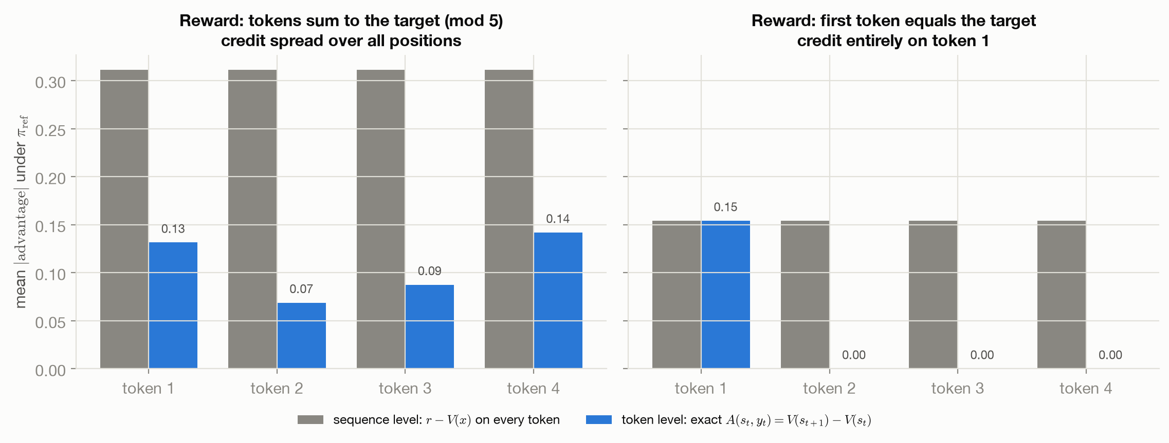
The two views give the same policy gradient, and the toy language shows why. With one terminal reward and \(\gamma = 1\), the token-level advantages telescope: \(\sum_t\big[V(s_{t+1}) - V(s_t)\big] = r(x,y) - V(x)\), the sequence-level advantage. They differ in how a single sample’s credit is distributed across its tokens. Figure 4.1 computes the exact per-token advantage \(A(s_t,y_t) = V^\pi(s_{t+1}) - V^\pi(s_t)\) under \(\pi_{\text{ref}}\) for two verifiable rewards. For the book’s default reward (the tokens sum to a target, mod 5), credit is spread over all four positions: the last token can always fix the sum, but \(\pi_{\text{ref}}\)’s choice of last token is far from uniform, so earlier tokens change the odds. For a reward decided by the first token, all the credit sits on token 1 and the other tokens carry none. The sequence-level view puts the same advantage, \(r - V(x)\), on every token in both cases. On average the excess pushes on irrelevant tokens cancel, but on any one sample they are noise. That noise is the credit-assignment problem in its LLM form, and critics, process rewards and dense teacher signals are each a way of getting closer to the blue bars.
Ahmadian et al. argue for the bandit view directly in their case for simpler RLHF methods: with a reward only at the end, “modeling partial sequences is an unnecessary undertaking”, and the whole completion can be treated as a single action (Ahmadian et al. 2024). Most of the critic-free methods in this book (RLOO, ReMax, GRPO) take that view, computing one advantage per response.
With a terminal reward and deterministic transitions, LLM fine-tuning against a reward model is a contextual bandit over whole responses (Sutton and Barto’s “associative search”), with a policy that happens to be factored autoregressively. Full MDP machinery (values of intermediate states, bootstrapping) is optional here, not required, which is why recipes could drop it.
4.2 Why this is an unusually easy and an unusually hard RL problem
ReMax names three properties of RLHF that distinguish it from classical deep RL (Li et al. 2023): fast simulation (“a trajectory … can be quickly obtained with minimal time overhead”), deterministic transitions (“the text context relies solely on past tokens and the presently generated token”), and trajectory-level rewards (“the reward model provides a single value only upon the completion of a response”). Together with the existence of a pretrained model, they make the problem easy in ways a robotics or games researcher would envy.
- The dynamics are known and deterministic. There is no model of the environment to learn and no stochastic transition to average over. Any state can be recreated for free by feeding its prefix, so “resetting” to an intermediate state is trivial.
- A strong prior policy already exists. RL does not start from random behavior. It starts from a pretrained and instruction-tuned model that already produces sensible responses and often correct ones. Ahmadian et al. point out that strong initialization leads to “the concentration of probability mass on a few tokens at each generation step”, even though the nominal action space is enormous, which keeps policy-gradient variance manageable (Ahmadian et al. 2024).
- Exploration mostly comes for free. Sampling from the prior, with some temperature, already covers plausible responses. Classical exploration bonuses rarely appear.
And it is hard in ways that classical RL rarely is.
- The action space is enormous. Tens of thousands of tokens per step, and \(|\mathcal{V}|^T\) possible responses. No exhaustive search or \(\arg\max\) over actions is possible at the response level.
- The reward is sparse. One number per response, possibly after thousands of tokens.
- The reward is often learned, and therefore hackable. A reward model is a proxy fitted to finite comparisons; a policy optimized against it will find its errors (the rewards chapter). Classical environments rarely have this problem: the score of an Atari game is the score.
- Sequences are long, so credit assignment is hard. Figure 4.1 in a four-token world becomes, in a thousand-token chain of thought, the question of which step of a long argument earned the reward.
- The policy must not drift far. The pretrained model’s knowledge and fluency are the point. Unlike an agent learning a game from scratch, an LLM being post-trained should change as little as it can while still improving, which is why every recipe is regularized toward \(\pi_{\text{ref}}\) in some way.
4.3 Classical RL vs. LLM-era RL
The easy and hard properties together predict which pieces of classical RL survived. The table records each concept’s classical meaning, what it became in LLM post-training, and why. It is revisited in the decision-guide chapter once every method has been covered.
| Concept | Classical meaning | In LLM post-training | Fate, and why |
|---|---|---|---|
| State | an environment state, often partially observed | prompt + generated prefix, fully observed | transformed: trivially Markov, but grows every step |
| Action | a small discrete set or a continuous vector | a token (token view) or a whole response (bandit view) | transformed: huge set, with a strong prior over it |
| Transition | unknown, stochastic, learned or sampled | known and deterministic: append the token | trivialized, until tools and environments return (agentic RL) |
| Reward | from the environment, often at every step | once per response, from a reward model, verifier or judge | transformed: sparse, and often learned and hackable |
| Discount \(\gamma\) | \(<1\), for infinite horizons and as a bias–variance knob | \(\gamma = 1\) on finite responses | discarded |
| Exploration | ε-greedy, optimism, intrinsic bonuses | sampling the pretrained prior at some temperature; entropy kept from collapsing (e.g. DAPO’s clip-higher) | transformed: inherited from pretraining rather than engineered |
| Value function / critic | central to value-based and actor–critic methods | a learned critic in PPO-based RLHF; dropped by RLOO, ReMax, GRPO | discarded in recent recipes: costs a model’s worth of memory, hard to train on sparse terminal rewards, and Monte Carlo baselines are cheap |
| Bootstrapping | TD targets, the bias–variance workhorse | little: with one terminal reward, Monte Carlo returns are available and cheap | mostly discarded |
| Off-policy learning | Q-learning from any behavior; importance sampling | “on-policy” with minibatch reuse; offline methods (DPO) learn from fixed data; asynchronous pipelines tolerate slightly stale samples (Noukhovitch et al. 2025) | transformed: kept close to on-policy, because large off-policy corrections are unstable |
| Trust region | TRPO, PPO | PPO’s clip, GRPO, and the sequence- and weight-level variants of 2025 | survived, central |
| KL to a reference | rare (entropy regularization is closer) | in nearly every objective, to \(\pi_{\text{ref}}\) | new in role: regularizes toward a prior, not just limiting a step |
| Experience replay | central to DQN-style methods | largely absent from policy optimization | mostly discarded: stale samples fight the trust region |
| Credit assignment | TD errors, eligibility traces, per-step rewards | one advantage broadcast to all tokens; critics, process rewards and dense teacher signals as partial fixes | open: the main unsolved problem the toy figure above illustrates |
Two entries deserve a comment. Bootstrapping, off-policy learning and function approximation are Sutton and Barto’s deadly triad (Sutton and Barto 2018, sec. 11.3), the combination with known instability. LLM recipes keep function approximation (unavoidably) and drop the other two almost entirely; whether or not that was the reason, it removes a classical source of divergence. And the “transition” row is the one most likely to change: when a model calls tools, browses or talks to a user over several turns, the environment is stochastic again, and the synthesis chapter discusses how the classical machinery returns.
4.4 The post-training pipeline
Where in training does RL happen, and why is it needed at all?
Pretraining fits \(\pi_\theta\) to a large corpus by next-token maximum likelihood: instructive feedback on a fixed dataset, supervised learning in the purest sense (the loss-functions-lab chapter on language-model objectives derives it).
Supervised fine-tuning (SFT, or instruction tuning) fits the model to demonstrations of the desired behavior, again by maximum likelihood. In RL terms this is behavior cloning: imitation learning on an expert’s trajectories, with the expert’s states as the training distribution. The first chapter described its known weakness. A policy trained only on the expert’s states makes errors on its own, those errors take it to states the expert never visited, and the cost can grow as \(T^2\epsilon\) rather than \(T\epsilon\) over a horizon of \(T\) (Ross and Bagnell 2010; Ross et al. 2011). For text, this is exposure bias (Ranzato et al. 2016). Instruction tuning works remarkably well anyway, but it has a ceiling it cannot get past on its own: it can only imitate, so it cannot learn what to do after its own mistakes, and it cannot exceed its demonstrations.
RL on the model’s own samples is the general remedy for both limitations. Training on states the policy itself visits removes the mismatch, which is DAgger’s insight (Ross et al. 2011); and evaluative feedback can reward behavior that no demonstrator wrote down. The preference and RL stages of post-training are where that happens.
Distillation, finally, transfers a large model’s behavior to a smaller one, either by SFT on the teacher’s outputs or on-policy, with the student generating and the teacher scoring (Learning by Imitating a Better Distribution).
SFT is behavior cloning. Its compounding-error problem is the one Ross and Bagnell analyzed, and the fix in imitation learning (DAgger) is to collect data on the learner’s own state distribution. RL on self-generated samples applies the same fix with evaluative feedback in place of expert labels.
The order pretrain → SFT → RL is the textbook pipeline, and it is the one InstructGPT made standard: demonstrations for SFT, then comparisons for a reward model, then PPO against it (Ouyang et al. 2022). Two cautions keep it from being taken as universal.
First, SFT before RL is not only about imitation. It also puts the policy in a region where RL can work at all: sampling must sometimes produce good responses for evaluative feedback to carry any signal (the hard prompt in the first chapter learned nothing until it did), and the output must be in a format the reward can read. Chu et al. report that “SFT stabilizes the model’s output format, enabling subsequent RL to achieve its performance gains” (Chu et al. 2025).
Second, real recipes are iterated and mixed. Tülu 3 runs SFT, then DPO, then RLVR, “a novel method we call Reinforcement Learning with Verifiable Rewards” (Lambert et al. 2024). DeepSeek-R1 is the canonical public example of interleaving: DeepSeek-R1-Zero applies RL (GRPO, with rule-based accuracy and format rewards) directly to a base model with no SFT at all; DeepSeek-R1 itself runs a small “cold-start” SFT, then reasoning-oriented RL, then rejection sampling to build a new SFT dataset, then SFT on it, then a second RL stage covering all scenarios (DeepSeek-AI 2025). RL outputs become SFT data; SFT checkpoints become RL starting points. There is no single canonical pipeline, only a toolbox of stages, each of which is one of the methods in Part III.
4.5 Connections
- Policy Gradients derived the token-level and sequence-level forms of the gradient; this chapter shows they are the same gradient with different credit assignment, and why recipes chose the sequence level.
- Where Rewards Come From, and How They Break takes up the “hard” property this chapter could only name: the reward is a learned proxy, and optimizing a proxy breaks it.
- Policy Gradients Without a Critic is the payoff of the bandit view: once the response is one action with one reward, a learned critic can be replaced by a Monte Carlo baseline from a group of samples.
- What RL Actually Does to a Model returns to the transition row of the table: multi-turn and agentic settings reintroduce real environment dynamics, and with them the classical machinery this chapter showed LLM recipes could drop.