6 The Shared Target, and RLHF with PPO
Part III derives the methods, and it starts not with a method but with a target. Almost every preference-learning and RL method used to post-train language models optimizes, exactly or approximately, the same objective: maximize reward while staying close, in KL divergence, to a reference policy. That objective has a closed-form optimum. Once it is written down, the method zoo stops looking like a zoo. PPO-based RLHF, DPO, rejection-sampling fine-tuning, critic-free policy gradients and on-policy distillation become different routes to one distribution, with different data, different estimators and different failure modes. This chapter derives the target, checks on the toy language that the routes really do arrive at it, and then walks the oldest and most expensive route, RLHF with PPO, which turns out to contain nothing that the earlier chapters have not already built.
6.1 The problem
The rewards chapter showed that maximizing a learned reward without restraint eventually destroys the true reward, and the first chapter showed that maximizing even a perfect reward collapses the policy onto a single answer. The standard fix, used since before RLHF had its name, is a KL penalty to a reference policy \(\pi_{\text{ref}}\) (usually the SFT model). Ziegler et al., the first to apply RL from human preferences to a pretrained language model, add “a penalty with expectation \(\beta\,\mathrm{KL}(\pi,\rho)\)” to keep the policy from moving too far from the pretrained model \(\rho\), “following Jaques et al.” (Ziegler et al. 2019), whose “KL-control” fine-tuned sequence models this way in 2017 (Jaques et al. 2017). The resulting objective is
\[ J_\beta(\pi) = \mathbb{E}_{x\sim\mathcal{D}_x}\Big[\,\mathbb{E}_{y\sim\pi(\cdot\mid x)}\big[r(x,y)\big] - \beta\,D_{\mathrm{KL}}\big(\pi(\cdot\mid x)\,\|\,\pi_{\text{ref}}(\cdot\mid x)\big)\Big]. \]
What policy maximizes it?
6.2 Assumptions
- The maximization is over all distributions \(\pi(\cdot\mid x)\) on responses, one per prompt. With a real network this is an idealization; on the toy language, whose policy is fully expressive, it is exact. Every claim below about “the optimum” is about this idealized problem, and every method has to be judged by how close it gets in practice.
- \(\pi_{\text{ref}}\) has full support where the reward matters. Responses that \(\pi_{\text{ref}}\) gives probability zero stay at zero.
- The reward is fixed during the optimization (a frozen reward model or verifier).
6.3 Derivation
Fix a prompt and drop \(x\). Expand the KL and collect everything inside one expectation under \(\pi\):
\[ J_\beta(\pi) = \sum_y\pi(y)\Big[r(y) - \beta\log\frac{\pi(y)}{\pi_{\text{ref}}(y)}\Big] = -\beta\sum_y\pi(y)\log\frac{\pi(y)}{\pi_{\text{ref}}(y)\,e^{r(y)/\beta}}. \]
The denominator is almost a distribution. Normalize it with \(Z = \sum_y\pi_{\text{ref}}(y)\,e^{r(y)/\beta}\), define \(\pi^\star(y) = \pi_{\text{ref}}(y)\,e^{r(y)/\beta}/Z\), and the objective becomes
\[ J_\beta(\pi) = -\beta\,D_{\mathrm{KL}}\big(\pi\,\|\,\pi^\star\big) + \beta\log Z . \]
\(\beta\log Z\) does not depend on \(\pi\), and a KL divergence is non-negative and zero only when the two distributions are equal. So the maximum is attained at \(\pi = \pi^\star\), and only there.
\[ \pi^\star(y\mid x) = \frac{1}{Z(x)}\,\pi_{\text{ref}}(y\mid x)\,\exp\!\big(r(x,y)/\beta\big), \qquad Z(x) = \sum_y \pi_{\text{ref}}(y\mid x)\,\exp\!\big(r(x,y)/\beta\big), \] and for every policy \(\pi\), \(\;J_\beta(\pi) = \mathbb{E}_x\big[\beta\log Z(x) - \beta\,D_{\mathrm{KL}}(\pi(\cdot\mid x)\,\|\,\pi^\star(\cdot\mid x))\big]\).
Two independent checks are in the test suite. Gradient ascent on the exact objective, which never uses the closed form, lands on \(\pi^\star\) to within \(10^{-6}\) nats; and the identity \(J_\beta = \beta\log Z - \beta D_{\mathrm{KL}}(\pi\|\pi^\star)\) holds for random policies to machine precision (tests/test_optimum.py).
The second line of the definition is as important as the first. Maximizing the KL-regularized reward is the same as minimizing the reverse KL from the policy to \(\pi^\star\). That is why the chapter on keeping updates stable cared so much about the direction of KL: RLHF is reverse-KL fitting of the policy to a fixed target, where SFT is forward-KL fitting to data.
Korbak, Perez and Buckley read the same algebra as Bayesian inference: \(\pi_{\text{ref}}\) is a prior, \(\exp(r/\beta)\) is the evidence, \(\pi^\star\) is the posterior, and the KL-regularized RL objective is “the evidence lower bound (ELBO)”, so that “KL-regularised RL is equivalent to variational inference” (Korbak et al. 2022). In classical RL this is the control-as-inference view, in which maximum-entropy RL “is equivalent to exact probabilistic inference in the case of deterministic dynamics” (Levine 2018). Text generation has deterministic dynamics, which is why the optimum here is a closed-form posterior rather than an approximation.
6.4 Interpretation
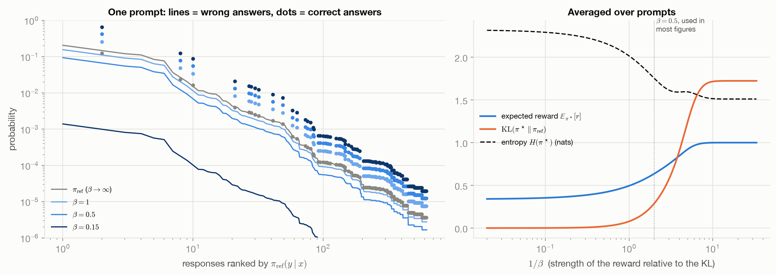
What does \(\pi^\star\) look like? It is the reference policy with every response’s probability multiplied by \(\exp(r/\beta)\) and renormalized. Figure 6.1 shows it for one prompt of the toy language. Every correct response is lifted by the same factor \(e^{1/\beta}\) relative to every wrong one; within the correct responses, and within the wrong ones, the reference policy’s own preferences are untouched. As \(\beta\to\infty\), \(\pi^\star\to\pi_{\text{ref}}\). As \(\beta\to0\), \(\pi^\star\) becomes \(\pi_{\text{ref}}\) restricted to the highest-reward responses: not a single answer, but the reference’s distribution over all of them. (Collapse onto one answer is a property of unregularized optimization dynamics, as in the first chapter, not of \(\pi^\star\).) Each \(\beta\) gives one point on the frontier of expected reward against KL, the gray curve that appears in many of this book’s figures.
Three consequences follow directly from the formula and recur in the next chapters.
- A per-prompt constant in the reward changes nothing. Adding \(c(x)\) to \(r\) multiplies the numerator and \(Z(x)\) by the same \(e^{c(x)/\beta}\). So the optimum is unaffected by the reward offset that a Bradley–Terry model cannot identify (the rewards chapter).
- The reward can be read off the optimal policy. Inverting the formula, \(r(x,y) = \beta\log\frac{\pi^\star(y\mid x)}{\pi_{\text{ref}}(y\mid x)} + \beta\log Z(x)\). DPO is built on this one line (the next chapter).
- Exact samples of \(\pi^\star\) can be drawn without training anything. Sample from \(\pi_{\text{ref}}\) and accept with probability \(e^{(r - r_{\max})/\beta}\): the accepted samples are distributed exactly as \(\pi^\star\) (rejection sampling; tested in
tests/test_optimum.py). Supervised fine-tuning on them is a route to \(\pi^\star\) that involves no gradient of the reward at all (Learning by Imitating a Better Distribution).
6.5 All roads lead to \(\pi^\star\)
With the target fixed, the method chapters can be previewed as routes to it.
| Route | How it reaches \(\pi^\star\) | Data | Chapter |
|---|---|---|---|
| PPO-based RLHF | on-policy policy gradient on \(r - \beta\log(\pi/\pi_{\text{ref}})\), learned critic, clipped trust region | fresh samples | this one |
| RLOO, GRPO | the same gradient with a Monte Carlo baseline from a group of samples instead of a critic | fresh samples | 8 |
| DPO | substitute the inverted formula into Bradley–Terry and fit \(\pi\) to preference pairs by logistic regression | a fixed dataset of pairs | 7 |
| Rejection-sampling fine-tuning | SFT on samples filtered to be distributed as \(\pi^\star\) | samples from \(\pi_{\text{ref}}\) | 9 |
| On-policy distillation | per-token reverse KL to a teacher that is (or approximates) \(\pi^\star\) | the student’s own samples | 9 |
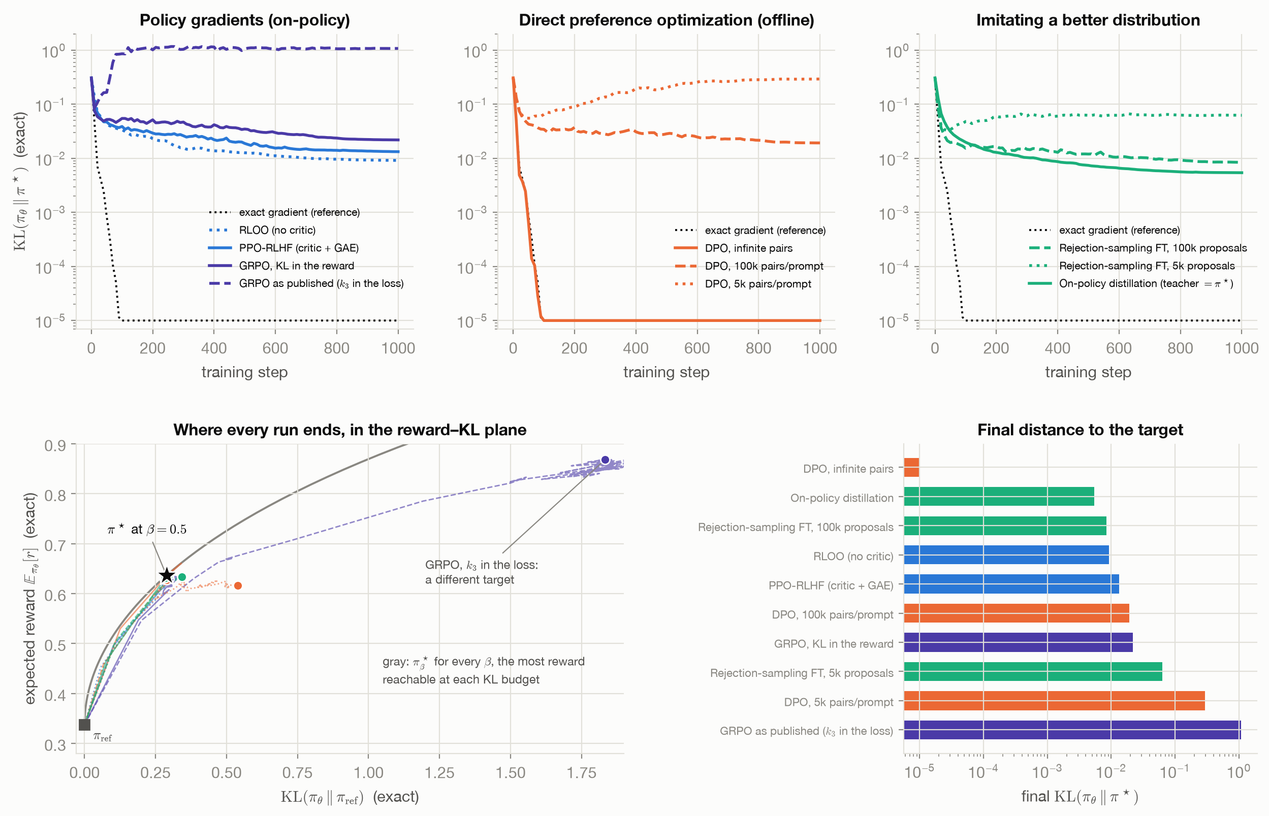
Figure 6.2 runs one representative of each route on the toy language with the same optimizer and learning-rate schedule and measures the exact KL from the trained policy to \(\pi^\star\). The top row groups the routes by family; the bottom row shows where each run ends.
The figure says three things, in increasing order of interest.
- The framework holds. DPO on its population loss (infinite preference pairs) reaches \(\pi^\star\) to machine precision, like the exact gradient, even though it never samples a response or evaluates a reward during training. The on-policy methods (RLOO, PPO with a critic, GRPO with the KL in the reward), on-policy distillation from \(\pi^\star\), and rejection-sampling fine-tuning on 100,000 proposals per prompt all end within about 0.005 to 0.02 nats of \(\pi^\star\).
- What separates them is the estimator. The on-policy methods stop at a noise floor set by their sampled gradients. The offline methods stop where their data runs out: DPO on 5,000 pairs per prompt first approaches \(\pi^\star\) and then drifts away to 0.29 nats, and rejection-sampling fine-tuning on 5,000 proposals plateaus at 0.06, because each converges to the optimum of its finite dataset rather than of the population. “Equivalent in the limit” is not “equivalent in practice”.
- Implementation details can change the target. GRPO as published puts its \(k_3\) KL estimator in the loss. The chapter on keeping updates stable showed that this regularizes the forward KL instead of the reverse one; here GRPO also divides each prompt’s advantages by their standard deviation while leaving the KL term unscaled, which further weakens the effective regularization (the same runs without the standard-deviation division end 0.49 nats from \(\pi^\star\) instead of 1.08, about half as far). It ends more than 1 nat from \(\pi^\star\), with much higher reward and a KL from \(\pi_{\text{ref}}\) six times larger. That is not a worse estimator of the same target; it is a different target. Policy Gradients Without a Critic takes it apart.
6.6 RLHF with PPO: the first route
The recipe that made the target practical is the one in Ziegler et al., Stiennon et al. and InstructGPT (Ziegler et al. 2019; Stiennon et al. 2020; Ouyang et al. 2022): collect comparisons, fit a Bradley–Terry reward model (the rewards chapter), then optimize \(J_\beta\) against it with PPO. It builds on Christiano et al., who learned the reward from comparisons in the same way but optimized it with A2C (Atari) and TRPO (simulated robotics), with no KL penalty toward a reference policy (Christiano et al. 2017). Seen from this book, every part of it has already been derived.
The reward, with the KL folded in. The KL term is implemented in the reward, per token. Ziegler et al. “perform RL on the modified reward \(R(x,y) = r(x,y) - \beta\log\frac{\pi(y\mid x)}{\rho(y\mid x)}\)” and either fix \(\beta\) or adapt it to hit a target KL (Ziegler et al. 2019); Stiennon et al. and InstructGPT do the same with \(\pi^{\text{SFT}}\) as the reference (Stiennon et al. 2020; Ouyang et al. 2022). Distributed over tokens, every step receives \(-\beta\log\frac{\pi(y_t\mid s_t)}{\pi_{\text{ref}}(y_t\mid s_t)}\) and the last step also receives \(r_\phi(x,y)\). This is the “\(k_1\) in the reward” implementation which, as the chapter on stable updates showed, follows the exact reverse-KL gradient and so targets \(\pi^\star\).
The episode. One response, one token per time step, \(\gamma = 1\) (Stiennon et al. 2020): the token-level MDP of the chapter on the LLM as a policy.
The critic, and where its targets come from. A value network \(V_\phi(s_t)\) predicts the return from each prefix. It is trained by regression toward returns computed from the sampled rollouts (with GAE, the advantage plus the old value estimate), and it supplies the baseline in the GAE advantages from the policy-gradient chapter. Stiennon et al. use “a Transformer with completely separate parameters from the policy” for it, initialized from the reward model, and InstructGPT initializes its value function from the reward model too (Stiennon et al. 2020; Ouyang et al. 2022).
The update. PPO’s clipped surrogate over several epochs of minibatches from each batch of rollouts, from the chapter on stable updates. InstructGPT adds a term that keeps fitting the pretraining distribution, “PPO-ptx”, with coefficient \(c_{\text{ptx}}\) (the paper’s \(\gamma\)), because it can “minimize performance regressions on public NLP datasets” (Ouyang et al. 2022).
| Signal | a learned reward model \(r_\phi(x,y)\) at the end of each response, minus \(\beta\log(\pi/\pi_{\text{ref}})\) at every token |
| Samples from (\(q\)) | \(\pi_{\text{old}}\): fresh rollouts each iteration, reused for a few epochs |
| Per-sample weight (\(w\)) | per token: \(\rho_t\hat A_t\) with GAE advantages, zeroed where the clip binds |
| Stability | KL to \(\pi_{\text{ref}}\) in the reward; ratio clipping; (optionally) a pretraining-likelihood term |
| Credit granularity | token level, through the critic and GAE |
| Models in memory | policy, reference, reward model, critic |
| Targets | the KL-regularized objective; its optimum \(\pi^\star\) (of the learned reward) |
| Classical lineage | PPO actor–critic with GAE, applied to the token-level MDP |
Running it on the toy language (rl4llm/methods/ppo.py, a tabular critic over prefixes) gives the “PPO-RLHF” curve of Figure 6.2: it reaches \(\pi^\star\) as well as the other on-policy methods, and no better.
Why four models, and why it is expensive and finicky. The policy is what is trained. The reference is needed at every step to compute the per-token KL. The reward model scores every rollout. The critic supplies token-level baselines. At LLM scale that is four large networks in memory, two of them trained, and generation inside the training loop. ReMax estimates that the value model alone takes about half of PPO’s GPU memory in RLHF (Li et al. 2023). The critic is also the hardest part to get right: it must predict a terminal reward from partial responses, on a distribution that moves every iteration, and an inaccurate critic biases every advantage (the GAE experiment in the policy-gradient chapter). With a single sequence-level reward, the bandit view of the LLM-as-policy chapter suggests the critic may not be worth its cost, which is the argument the critic-free methods make.
Nothing in PPO-based RLHF is new as RL: an actor–critic policy gradient with GAE advantages and a clipped trust region, on an MDP whose dynamics are trivial and whose reward function is a learned network. What is specific to LLMs is the per-token KL penalty to a frozen reference policy, which is what gives the whole procedure its closed-form target.
6.7 Behavior and failure modes
The target is only as good as the reward. \(\pi^\star\) is defined by \(r\). With a learned reward model it is the optimum of the proxy, and the rewards chapter traced exactly that family of distributions, \(\pi^\star_\beta(\text{proxy})\), as the curve along which the true reward peaks and falls. The KL term limits how far along that curve training goes; it does not make the proxy right.
Reaching the optimum is not the same as optimizing the objective. Every route in Figure 6.2 optimizes something whose optimum is \(\pi^\star\), but each stops somewhere else, for its own reason. When two methods “optimize the same objective”, the useful questions are how close each gets, and why it stops where it does.
The objective has a temperature, and its meaning depends on the reward’s scale. \(\pi^\star\) depends on \(r/\beta\), so the same \(\beta\) is a different regularizer for a reward model trained on sharper or noisier preferences, and for a GRPO run that normalizes its advantages.
6.8 Connections
- Keeping Updates Stable supplied PPO, the direction of the KL, and the reason the KL’s implementation matters; this chapter shows the objective is reverse-KL fitting to \(\pi^\star\).
- Direct Preference Methods inverts the closed form to express the reward through the policy and removes the reward model and the RL loop altogether.
- Policy Gradients Without a Critic keeps this chapter’s on-policy route but replaces its most expensive part, the critic, with a group of samples.
- Learning by Imitating a Better Distribution develops the routes that sample from (an approximation of) \(\pi^\star\) and then imitate it.