3 Keeping Updates Stable
The policy gradient is unbiased only for samples drawn from the current policy. That makes it expensive: every batch of responses, which for a language model means a full round of generation, can be used for exactly one gradient step before the policy changes and the batch goes stale. It also makes it fragile, in a way supervised learning never is. In supervised learning a bad step is a bad step: the data stays where it was, and the next gradient points back. In RL the policy chooses its own data, so a bad step changes which data the learner sees next, and a policy that has collapsed onto bad behavior may never again generate the samples that would show it the way back. This chapter covers the two families of tools LLM post-training inherited for this problem. Trust regions let a batch be reused for several steps while limiting how far the policy can move. KL penalties keep the policy near a reference distribution for the whole of training. Along the way it separates two things that share the letters “KL” and are easily confused: a KL to the previous policy, which limits the step size, and a KL to a fixed reference, which changes the objective. It also shows that how a KL penalty is implemented decides which divergence is actually being regularized.
3.1 The problem
Two problems, really, with the same root.
- Sample reuse. Generation dominates the cost of RL for language models. We would like to take several gradient steps on each batch, but after the first step the batch comes from \(\pi_{\text{old}}\), not from \(\pi_\theta\), and the plain policy gradient is no longer correct.
- Step size. Even with fresh samples, a step that is too large in parameter space can be enormous in policy space. Because the next batch is drawn from the new policy, an overshoot is not corrected by the next gradient the way it would be in supervised learning; it changes the data the next gradient is computed on.
The root is the property from the first chapter: the data distribution moves with the learner.
3.2 Reusing a batch: importance ratios
Importance sampling corrects for sampling from the wrong distribution. For any function \(f\), \(\mathbb{E}_{y\sim\pi_\theta}[f(y)] = \mathbb{E}_{y\sim\pi_{\text{old}}}\big[\tfrac{\pi_\theta(y)}{\pi_{\text{old}}(y)}f(y)\big]\). Applied to advantages at the token level, with the importance ratio \(\rho_t(\theta) = \pi_\theta(y_t\mid s_t)/\pi_{\text{old}}(y_t\mid s_t)\), this gives the surrogate objective
\[ L^{\text{CPI}}(\theta) = \hat{\mathbb{E}}_t\big[\,\rho_t(\theta)\,\hat A_t\,\big], \]
where \(\hat{\mathbb{E}}_t\) averages over the tokens of a batch sampled from \(\pi_{\text{old}}\) (the name is from the conservative policy iteration literature that Schulman et al. build on). At \(\theta = \theta_{\text{old}}\) every ratio is 1 and \(\nabla_\theta\rho_t = \nabla_\theta\log\pi_\theta(y_t\mid s_t)\), so the surrogate’s gradient is the policy gradient. Away from \(\theta_{\text{old}}\) it is only an approximation: it reweights the actions that were taken but still evaluates them in the states \(\pi_{\text{old}}\) visited, and the advantages were estimated for \(\pi_{\text{old}}\). Maximizing it without limit would drive the ratios of positive-advantage tokens to infinity. The approximation is good only while \(\pi_\theta\) stays close to \(\pi_{\text{old}}\). That is the reason for a trust region.
3.3 Trust regions: TRPO
Schulman et al.’s Trust Region Policy Optimization proved that the true objective is bounded below by the surrogate minus a penalty proportional to the largest per-state KL between old and new policy, so maximizing the penalized surrogate at every iteration guarantees “a monotonically improving sequence of policies” (Schulman et al. 2015, secs. 3–4). The penalty coefficient that the theory requires gives tiny steps, so the practical algorithm replaces it with a constraint, and the maximum over states with an average:
\[ \max_\theta\; \hat{\mathbb{E}}_t\big[\rho_t(\theta)\hat A_t\big] \quad\text{subject to}\quad \mathbb{E}_{s\sim\pi_{\text{old}}}\big[D_{\mathrm{KL}}\big(\pi_{\text{old}}(\cdot\mid s)\,\|\,\pi_\theta(\cdot\mid s)\big)\big]\le\delta . \]
The paper calls the averaged constraint “a heuristic approximation” to the bound and used \(\delta = 0.01\) in all its experiments (Schulman et al. 2015, secs. 4, 8). Solving it takes a conjugate-gradient step on a second-order approximation of the KL and a line search, which is why TRPO was rarely used at LLM scale.
The idea comes from numerical optimization: trust a local model of the objective only in a neighborhood of the current point, and choose the step by optimizing the model within that neighborhood. TRPO measures the neighborhood in policy space (KL between action distributions) rather than parameter space, which is what makes it meaningful for RL.
3.4 PPO’s clipped surrogate
Proximal Policy Optimization keeps the idea and drops the second-order machinery. Its main variant replaces the constraint with a clip inside the objective (Schulman et al. 2017, eq. 7):
\[ L^{\text{CLIP}}(\theta) = \hat{\mathbb{E}}_t\Big[\min\big(\rho_t(\theta)\hat A_t,\;\mathrm{clip}(\rho_t(\theta),\,1-\epsilon,\,1+\epsilon)\,\hat A_t\big)\Big],\qquad \epsilon \approx 0.2 . \]
The authors describe it exactly: clipping “removes the incentive for moving \(r_t\) outside of the interval \([1-\epsilon, 1+\epsilon]\)”, and taking the minimum makes the result “a lower bound (i.e., a pessimistic bound) on the unclipped objective”, so that “we only ignore the change in probability ratio when it would make the objective improve, and we include it when it makes the objective worse” (Schulman et al. 2017, sec. 3). With this objective the same batch is optimized for \(K\) epochs of minibatch updates (usually with Adam).
Figure 3.1 plots one token’s term and its derivative with respect to the ratio. There are four regions. With a positive advantage, the gradient is the full \(\hat A_t\) until the ratio exceeds \(1+\epsilon\), and zero beyond it: the token has already been made \(\epsilon\) more likely, and there is no reward for pushing it further on this batch. With a negative advantage the mirror image holds below \(1-\epsilon\). In the other two corners, where the ratio has moved the wrong way (a good token became less likely, a bad token more likely), the minimum picks the unclipped term, the full gradient is kept, and the mistake can be undone. The clip is one-sided by design.
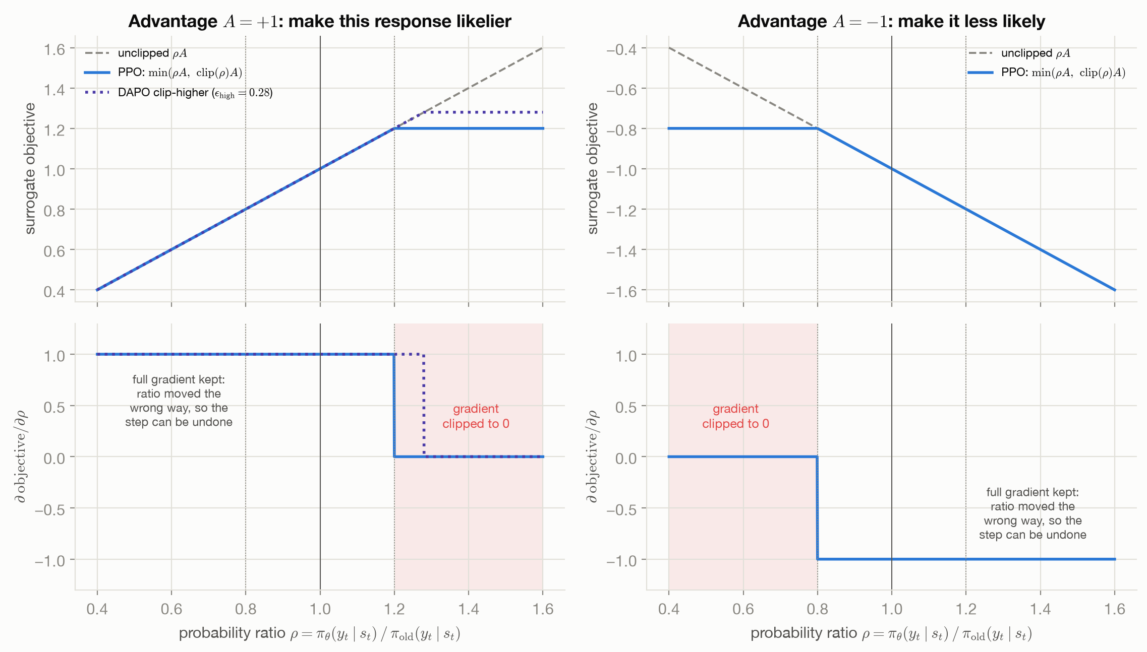
Two details matter later. The clip is applied per token, so an LLM response contains a mix of clipped and unclipped tokens; Policy Gradients Without a Critic shows that low-probability tokens, whose ratios swing most, are the ones most often clipped, and how DAPO, GSPO and CISPO each change this. And PPO is a slightly off-policy method: within an iteration it optimizes on samples from \(\pi_{\text{old}}\). When LLM papers call PPO or GRPO “on-policy”, this is what they mean.
The full PPO objective adds a value-function loss for the critic and an entropy bonus: \(L^{\text{CLIP}} - c_1 L^{\text{VF}} + c_2 S[\pi_\theta]\) (Schulman et al. 2017, eq. 9). The paper also gives an alternative, the adaptive KL penalty, which subtracts \(\beta\,\mathrm{KL}[\pi_{\text{old}}(\cdot\mid s_t),\pi_\theta(\cdot\mid s_t)]\) and adapts \(\beta\) to hit a target KL; the authors report that it “performed worse than the clipped surrogate objective” (Schulman et al. 2017, sec. 4). Note which KL that is: to \(\pi_{\text{old}}\), the policy that generated the batch. It is a soft trust region, not a pull toward a fixed prior.
| Signal | scalar reward from the environment, per step |
| Samples from (\(q\)) | \(\pi_{\text{old}}\): one batch reused for \(K\) epochs of minibatches (slightly off-policy) |
| Per-sample weight (\(w\)) | per token: \(\rho_t\hat A_t\), with the gradient zeroed where the clip binds |
| Stability | ratio clipping (a soft trust region); optional adaptive KL to \(\pi_{\text{old}}\); entropy bonus |
| Credit granularity | per step, from a learned critic via GAE |
| Models in memory | policy, value function |
| Targets | expected return; no reference policy |
| Classical lineage | TRPO’s trust region, simplified; actor–critic with GAE |
3.5 KL, entropy, and the direction of divergence
PPO’s own regularizers are local: the clip and the optional KL to \(\pi_{\text{old}}\) limit each step, and the entropy bonus discourages premature determinism. LLM post-training adds something of a different kind, a KL to a fixed reference policy \(\pi_{\text{ref}}\), usually the SFT model, that stays in the objective for the whole run:
\[ \max_\theta\;\mathbb{E}_{x,\;y\sim\pi_\theta}\big[r(x,y)\big] - \beta\,D_{\mathrm{KL}}\big(\pi_\theta(\cdot\mid x)\,\|\,\pi_{\text{ref}}(\cdot\mid x)\big). \]
This term changes what is being optimized, not just how fast. It bounds how far the final policy can drift from the reference, however long training runs. The shared-target chapter shows that it gives the objective a closed-form optimum, \(\pi^\star\propto\pi_{\text{ref}}\exp(r/\beta)\), the hub of this book. Stiennon et al. gave two reasons for it in the RLHF setting: it “acts as an entropy bonus, encouraging the policy to explore and deterring it from collapsing to a single mode”, and it keeps the policy from producing outputs too different from those the reward model was trained on (Stiennon et al. 2020). The first reason is a cousin of PPO’s entropy bonus: since \(D_{\mathrm{KL}}(\pi\|\pi_{\text{ref}}) = -H(\pi) - \mathbb{E}_\pi[\log\pi_{\text{ref}}]\), the penalty rewards entropy, but entropy measured relative to the reference rather than relative to uniform.
Which direction, and why it matters
KL divergence is not symmetric, and the two directions ask for different things. \(D_{\mathrm{KL}}(p\|q) = \mathbb{E}_p[\log p/q]\) is large wherever \(p\) has mass and \(q\) does not. Minimizing it over \(q\) (the forward KL, which is what maximum likelihood does with \(p\) the data distribution) forces \(q\) to cover everything \(p\) covers: it is mass-covering. \(D_{\mathrm{KL}}(q\|p)\) is large wherever \(q\) has mass and \(p\) does not. Minimizing it (the reverse KL) forces \(q\) to stay inside \(p\)’s support but lets it ignore parts of \(p\): it is mode-seeking. Figure 3.2 shows the difference by fitting a single Gaussian to a target with two modes.
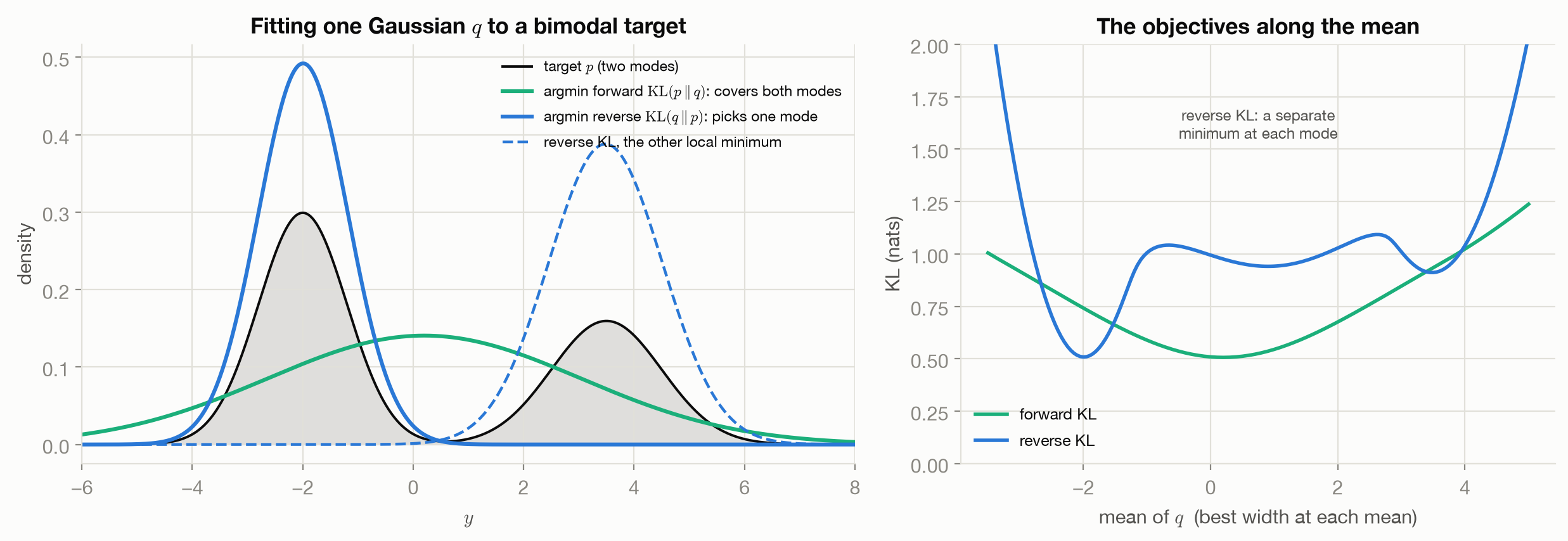
The KL-regularized RL objective uses the reverse direction, \(D_{\mathrm{KL}}(\pi_\theta\|\pi_{\text{ref}})\), and the shared-target chapter shows that the whole objective equals \(-\beta D_{\mathrm{KL}}(\pi_\theta\|\pi^\star)\) plus a constant: training is reverse-KL fitting of the policy to \(\pi^\star\). Supervised fine-tuning, by contrast, minimizes the forward KL from the data to the model. Two cautions keep this from becoming a slogan. With a policy expressive enough to represent \(\pi^\star\) exactly, as on the toy language, the reverse-KL optimum is \(\pi^\star\), which keeps every response \(\pi_{\text{ref}}\) supports; mode-seeking bites when the policy cannot represent the target, when optimization stops early, and in the limit \(\beta\to0\) where the KL term vanishes. And with no KL term at all, reward maximization is the extreme case: the first chapter showed REINFORCE collapsing onto a single correct answer while SFT on the same task kept the expert’s spread. The synthesis chapter returns to what this means for the diversity of trained models.
3.6 Estimating a KL, and regularizing with one
In practice \(D_{\mathrm{KL}}(\pi_\theta\|\pi_{\text{ref}})\) is never computed exactly; it is estimated from the sampled responses. Schulman’s note on approximating KL divergence defines three single-sample estimators for samples \(y\sim\pi_\theta\) with \(u = \pi_{\text{ref}}(y)/\pi_\theta(y)\) (the note writes \(r\); here \(r\) is always a reward) (Schulman 2020):
- \(k_1 = -\log u\): unbiased, but noisy and negative for some samples;
- \(k_2 = \tfrac12(\log u)^2\): always non-negative and low-variance, but biased (its mean is a different f-divergence that matches the KL only to second order);
- \(k_3 = (u-1) - \log u\): unbiased and always non-negative, by adding the zero-mean control variate \(u - 1\) to \(k_1\).
GRPO uses \(k_3\), per token, and calls it “unbiased” and “guaranteed to be positive” (Shao et al. 2024, sec. 4.1). The top row of Figure 3.3 checks these properties on the toy language, exactly, along a path of policies moving away from \(\pi_{\text{ref}}\). As a value, \(k_1\) and \(k_3\) are unbiased and \(k_2\) is not. In noise, \(k_3\) is much better than \(k_1\) near \(\pi_{\text{ref}}\), but not far from it: its relative standard deviation grows as the policy moves, because the ratio \(\pi_{\text{ref}}/\pi_\theta\) is heavy-tailed under \(\pi_\theta\), and beyond a KL of about 0.5 it is noisier than \(k_1\). (Schulman’s own check used two Gaussians with KLs of 0.005 and 0.5, the regime where \(k_3\) wins.)
An unbiased value is not an unbiased gradient
The more consequential question is what happens when an estimator is differentiated. There are two ways to put a KL penalty into training, and they are not equivalent.
KL in the reward. Subtract \(\beta\log(\pi_\theta/\pi_{\text{ref}})\) from each sample’s reward and use the score function as usual. This is classic RLHF: the per-token reward \(r_t = r_\phi - \beta\log\frac{\pi_\theta(y_t\mid s_t)}{\pi_{\text{ref}}(y_t\mid s_t)}\) in InstructGPT-style PPO (Ouyang et al. 2022; Shao et al. 2024). Its expected gradient is \(\mathbb{E}_{\pi_\theta}[\log(\pi_\theta/\pi_{\text{ref}})\nabla\log\pi_\theta]\), which is exactly \(\nabla D_{\mathrm{KL}}(\pi_\theta\|\pi_{\text{ref}})\); the extra \(-\mathbb{E}[\nabla\log\pi_\theta]\) term vanishes by the zero-mean score of the previous chapter.
KL as a loss. Compute an estimate \(k(y)\) for each sample and add \(\beta\cdot\mathrm{mean}(k)\) to the loss, differentiating it directly with the samples held fixed. GRPO does this, for a reason the paper states: “instead of adding KL penalty in the reward, GRPO regularizes by directly adding the KL divergence between the trained policy and the reference policy to the loss, avoiding complicating the calculation of \(\hat A_{i,t}\)” (Shao et al. 2024, sec. 4.1.1). Keeping the KL out of the advantage keeps it out of the group normalization. But differentiating an estimator with the samples held fixed ignores that the samples themselves depend on \(\theta\), so the resulting gradient need not be the gradient of what was estimated. Working it out for each estimator (each is a function of \(\log\pi_\theta(y)\), so its pathwise derivative is a weight on \(\nabla\log\pi_\theta(y)\)):
| Implementation | Expected gradient (on-policy) | What it regularizes |
|---|---|---|
| \(k_1\) in the reward | \(\mathbb{E}_{\pi_\theta}[\log\frac{\pi_\theta}{\pi_{\text{ref}}}\nabla\log\pi_\theta]\) | reverse KL \(D_{\mathrm{KL}}(\pi_\theta\|\pi_{\text{ref}})\) |
| \(k_2\) as a loss | the same | reverse KL |
| \(k_1\) as a loss | \(\mathbb{E}_{\pi_\theta}[\nabla\log\pi_\theta] = 0\) | nothing |
| \(k_3\) as a loss | \(\mathbb{E}_{\pi_\theta}[(1-\frac{\pi_{\text{ref}}}{\pi_\theta})\nabla\log\pi_\theta] = -\sum_y\pi_{\text{ref}}\nabla\log\pi_\theta\) | forward KL \(D_{\mathrm{KL}}(\pi_{\text{ref}}\|\pi_\theta)\) |
The last line deserves the algebra: \(\sum_y\pi_\theta(1-\pi_{\text{ref}}/\pi_\theta)\nabla\log\pi_\theta = \sum_y\pi_\theta\nabla\log\pi_\theta - \sum_y\pi_{\text{ref}}\nabla\log\pi_\theta = 0 + \nabla_\theta D_{\mathrm{KL}}(\pi_{\text{ref}}\|\pi_\theta)\). Two 2025 analyses reach the same conclusions from different directions. Liu et al. show that “\(k_1\) in reward” and “\(k_2\) as loss” are gradient-equivalent on-policy, that “\(k_1\) as loss” has zero expected gradient, and that “\(k_3\) as loss” is “a first-order, biased approximation” of the principled reverse-KL gradient (Liu et al. 2025). Zhang et al. show that \(k_3\)’s expectation is the reverse KL, and that GRPO’s KL term lacks the importance weight \(\pi_\theta/\pi_{\text{old}}\) that would make its gradient follow it when samples come from \(\pi_{\text{old}}\) (Zhang et al. 2026). The table is the on-policy case of both. The test suite checks all four rows against finite differences on the toy language (tests/test_kl_penalties.py).
The bottom row of Figure 3.3 shows what this does to training. Each run maximizes the reward with exact gradients and a penalty of strength \(\beta = 0.5\) implemented one of the five ways. Only \(k_1\) in the reward and \(k_2\) as a loss converge to \(\pi^\star\). Sequence-level \(k_3\) as a loss converges to a different policy, with more reward (0.71 vs 0.64) and about twice the reverse KL from \(\pi_{\text{ref}}\) (0.56 vs 0.29). The per-token version, as GRPO implements it, drifts further (1.07). \(k_1\) as a loss regularizes nothing, and the policy collapses onto correct answers as if \(\beta\) were zero.
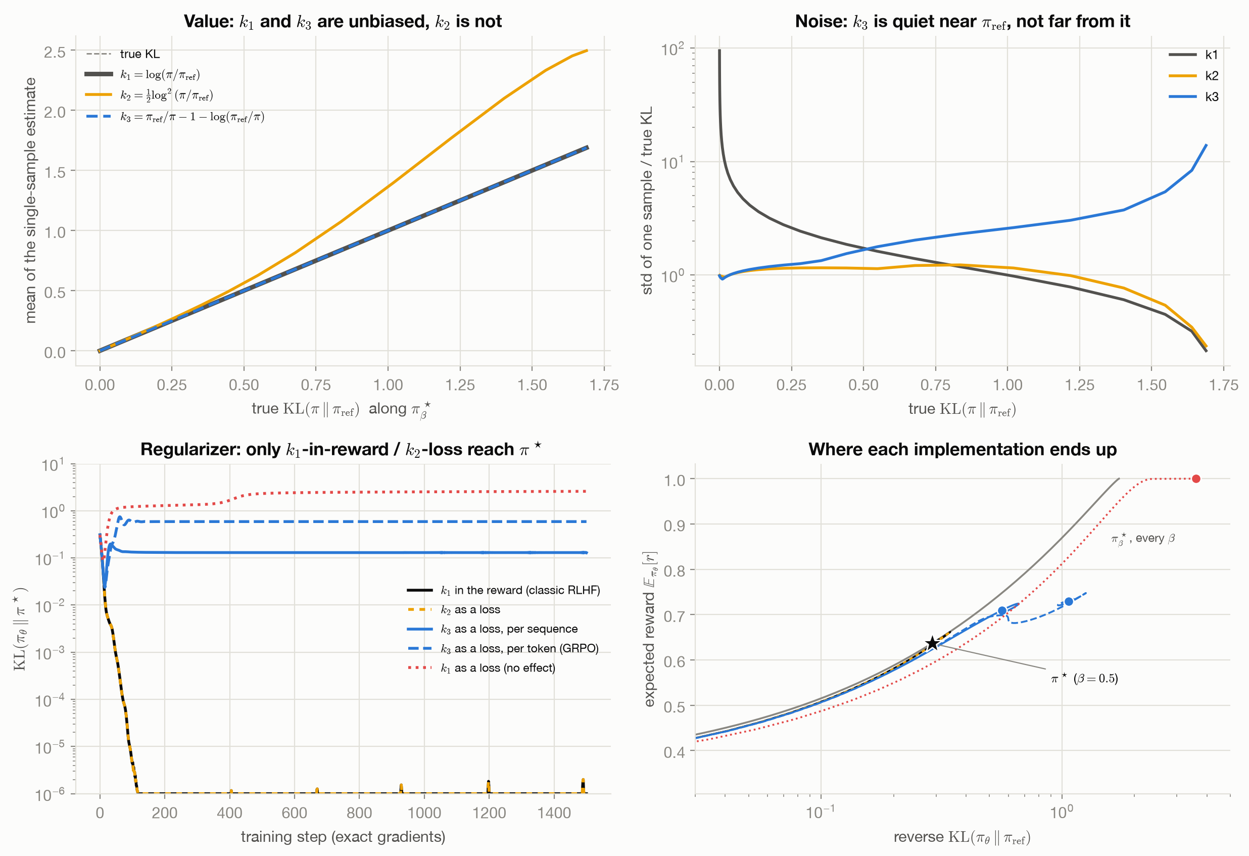
How much this matters in practice is a separate question, and the toy cannot settle it. Real GRPO training also clips, samples finitely, normalizes advantages and uses a small coefficient (DeepSeekMath used \(\beta = 0.04\) (Shao et al. 2024, sec. 4.2)), and several recent recipes drop the KL term altogether (DAPO does, arguing that “the model distribution can diverge significantly from the initial model” in long chain-of-thought training (Yu et al. 2025)). What the toy does establish is a mathematical fact: the estimator and its placement decide which divergence is regularized, and therefore what the target of training is. An estimator chosen for being unbiased as a value is not thereby a correct regularizer.
The difference between “KL in the reward” and “KL as a loss” is the classical distinction between two ways to differentiate an expectation: the score-function (likelihood-ratio, REINFORCE) estimator, which accounts for how the sampling distribution moves with \(\theta\), and the pathwise derivative, which differentiates the integrand with the samples held fixed. For a discrete policy only the score function is unbiased in general; a pathwise term is correct only when the integrand’s dependence on \(\theta\) has been accounted for, which is what the importance weight in Zhang et al.’s correction does.
3.7 Interpretation
Each mechanism in this chapter controls something different, and LLM recipes combine them.
- The importance ratio lets a batch be reused, and is accurate only near \(\pi_{\text{old}}\).
- The clip (or TRPO’s constraint, or a KL to \(\pi_{\text{old}}\)) limits how far one iteration can move the policy. It changes the optimization path, not the destination.
- The KL to \(\pi_{\text{ref}}\) changes the destination: the optimum of the regularized objective is \(\pi^\star\), not the reward maximizer.
- The implementation of that KL decides whether the destination really is \(\pi^\star\).
3.8 Behavior and failure modes
Clipping hides problems instead of solving them. A clipped token contributes no gradient, so if the advantage estimates are wrong, or a few tokens’ ratios explode, the clip silences them rather than flagging them. Monitoring the fraction of clipped tokens is the usual diagnostic.
The trust region is token-level; the reward is sequence-level. A sequence-level change in probability is the product of many per-token ratios, each within \(1\pm\epsilon\), which can still be a large change for the sequence. GSPO’s sequence-level ratio is a response to this mismatch (Policy Gradients Without a Critic).
A KL penalty is not a guarantee against a bad reward. It limits drift from \(\pi_{\text{ref}}\) but does not distinguish good drift from reward hacking. Gao et al. found that varying the KL penalty mostly changes where along the gold-reward-vs-KL curve training stops (the rewards chapter).
Estimators can silently change the target. The table above.
3.9 Connections
- Policy Gradients supplies the on-policy gradient that importance ratios correct and the advantages that the clip multiplies.
- The Shared Target, and RLHF with PPO derives the closed-form optimum that the KL-to-reference term creates, and assembles this chapter’s PPO with a critic, a reward model and the per-token KL in the reward into the RLHF recipe.
- Policy Gradients Without a Critic revisits the clip (DAPO’s clip-higher, GSPO’s sequence-level ratio, CISPO’s clipped weights) and GRPO’s KL term, now that the difference between KL in the reward and KL in the loss is clear.
- Where Rewards Come From, and How They Break shows what the KL penalty does and does not protect against when the reward is a learned proxy.