1 What Makes a Problem RL
Most of us met reinforcement learning as a separate subject. It arrived with its own vocabulary (agents, environments, MDPs, Bellman equations, Q-tables, exploration) and its own canonical examples (gridworlds, Atari, Go), and it was easy to come away believing that RL is a different kind of machine learning, with different models and different losses. Then language-model post-training started calling things RL that look, from the outside, like fine-tuning a transformer with a slightly unusual loss. Both impressions are half right. This chapter makes the boundary precise. The claim it defends is the first thesis of the book: RL is defined by where the training data comes from and what kind of feedback it carries, not by the model or the loss. Once that is clear, the rest of the classical apparatus (returns, values, the Bellman equation, the split between value-based and policy-based methods) can be introduced as answers to specific problems that this kind of feedback creates, rather than as a separate world.
1.1 Three kinds of feedback
Take one model and put it in three situations.
A classifier. An image comes in, the model outputs a distribution over labels, and a dataset tells it the correct label. Training pushes up the log-probability of that label. Note two things about the signal. It says what the right answer was, regardless of what the model predicted. And the images arrive from a fixed dataset that has nothing to do with the model’s current behavior.
A recommender that shows one item. A user arrives, the model picks one article to show, and the system observes whether the user clicked. Now the signal is different in kind. A click on article 3 says that article 3 was good enough to click. It says nothing about articles 1, 2 or 4, which were never shown. And which article got shown, and therefore which piece of feedback exists at all, was decided by the model itself. This is the setting Li et al. formalized as a contextual bandit for news recommendation (Li et al. 2010).
A game. The model makes a move, then another, then forty more, and at the end it learns whether it won. Now there is a third difficulty: the outcome cannot be traced to any single move. Some early move might have lost the game; the final move might have been brilliant. The feedback is delayed, and credit has to be spread across the sequence somehow.
Sutton and Barto put the first distinction at the center of their textbook: “the most important feature distinguishing reinforcement learning from other types of learning is that it uses training information that evaluates the actions taken rather than instructs by giving correct actions” (Sutton and Barto 2018, ch. 2). Instructive feedback, they write, “indicates the correct action to take, independently of the action actually taken”; evaluative feedback “indicates how good the action taken was, but not whether it was the best or the worst action possible”. Their opening chapter names the second and third distinctions as well: “trial-and-error search and delayed reward” are “the two most important distinguishing features of reinforcement learning” (Sutton and Barto 2018, sec. 1.1). The three situations above are those three properties, switched on one at a time.
- Instructive vs. evaluative feedback. A label says what the right answer was. A reward says only how good the answer you gave was, and nothing about the answers you did not give.
- Fixed vs. self-generated data. In supervised learning the data distribution is given. In RL the learner’s own policy decides which data it sees, so the training distribution moves as the learner changes.
- Immediate vs. delayed consequences. Either a reward can be traced to the action that caused it, or credit must be spread across a sequence of actions.
Placing the familiar problem types in this space gives the following table.
| Feedback | Data | Consequences | |
|---|---|---|---|
| Supervised learning | instructive | fixed | immediate |
| Contextual bandit | evaluative | self-generated | immediate |
| Full RL (MDP) | evaluative | self-generated | delayed |
| Imitation learning / SFT | instructive | fixed (the expert’s distribution, not the learner’s) | delayed at test time |
The contextual bandit sits exactly between supervised learning and full RL. Sutton and Barto call it associative search and describe it the same way: like full RL “in that [it involves] learning a policy”, but like a bandit “in that each action affects only the immediate reward. If actions are allowed to affect the next situation as well as the reward, then we have the full reinforcement learning problem” (Sutton and Barto 2018, sec. 2.9).
The last row deserves a second look, because it is where language-model training starts. Imitation learning, and its LLM incarnation supervised fine-tuning (SFT), trains on instructive feedback from a fixed dataset of an expert’s behavior. During training it looks exactly like supervised learning. At test time, however, the learner acts in a sequence, and its own earlier actions decide which situations it ends up in. If it makes a mistake it reaches states the expert never visited, where it was never trained, and errors compound. Ross and Bagnell made this quantitative: a policy that errs with probability \(\epsilon\) on the expert’s state distribution can incur a cost that grows as \(T^2\epsilon\) over a horizon of \(T\) steps, rather than \(T\epsilon\), and the bound is tight (Ross and Bagnell 2010; Ross et al. 2011). In sequence generation the same mismatch has a name of its own, exposure bias: Ranzato et al. used it for “a model [that] is only exposed to the training data distribution, instead of its own predictions” (Ranzato et al. 2016). Their remedy, notably, was to train the text generator on its own samples with REINFORCE, years before RLHF. The general remedy for training on someone else’s distribution is to train on your own, which is the second property in the list above.
So the “RL is a different category” intuition is half true. As the rest of this chapter shows, the mathematics is mostly shared. What really differs is the data-generating process.
1.2 One model, one gradient, three signals
The claim that only the signal differs can be tested directly. The book’s experiments run on a small enumerable language (described in the testbed appendix): five tokens, responses of exactly four tokens, so \(5^4 = 625\) possible responses, and four prompts. A reference policy \(\pi_{\text{ref}}\) was fit by maximum likelihood to a synthetic corpus, and a response is correct if its tokens sum to the prompt’s target modulo 5, a toy version of a verifiable math answer. Because there are only 625 responses, the probability that the current policy answers correctly can be computed exactly at every step rather than estimated.
Starting from \(\pi_{\text{ref}}\), the same policy is trained three ways, with the same optimizer and learning rate, and with the same final operation: a gradient step on \(\sum_i w_i \log\pi_\theta(y_i\mid x_i)\) over a batch of responses \(y_i\). Only the responses and the weights differ.
- Instructive: the batch is demonstrations, correct answers drawn from an expert (here, \(\pi_{\text{ref}}\) restricted to correct responses), each with weight 1. This is supervised learning, or SFT.
- Evaluative, self-generated: the batch is the policy’s own samples, weighted by their reward minus the average reward of the other samples for the same prompt. This is REINFORCE, the basic policy-gradient algorithm the next chapter derives.
- Evaluative, fixed log: the batch is samples that \(\pi_{\text{ref}}\) generated (a log of someone else’s behavior), weighted by their reward. Responses that happened to be correct get pushed up; nothing else does.
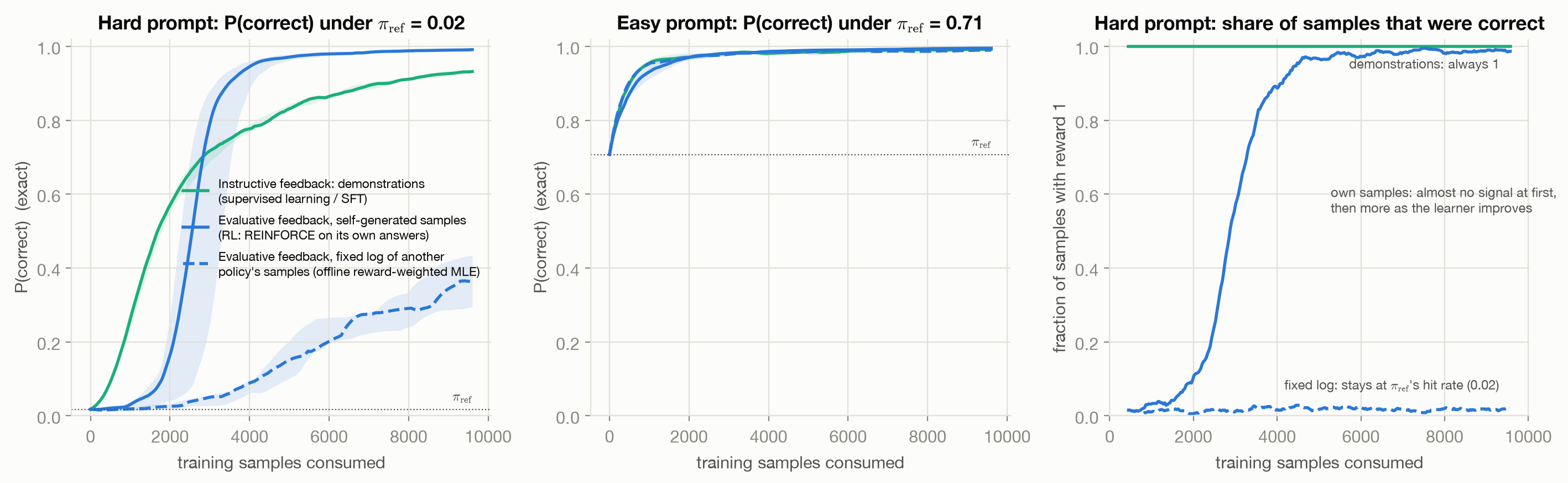
Figure 1.1 shows the three runs. On the easy prompt all three behave almost identically: when most answers are already right, it hardly matters whether the signal says “this is correct” or “this one scored 1”. The hard prompt separates them, and each difference traces back to one of the properties in the table.
Demonstrations are informative from the first step, because instructive feedback does not depend on what the learner currently does. The learner’s own samples carry almost no signal at first: with a 2% hit rate, most groups of eight answers contain no correct answer at all, every reward is zero, and the gradient is zero. Evaluative feedback cannot tell the learner what it should have said. Once a few correct answers have been reinforced, the policy produces more of them, its batches become informative, and learning accelerates sharply (the right panel). That acceleration is the self-generated property at work. The fixed log has the same evaluative signal but no such feedback loop: the share of useful samples stays at \(\pi_{\text{ref}}\)’s 2% forever, and after the same number of samples the policy is still right only about 36% of the time (median over the five seeds; 29% to 43%).
The figure also shows something the table did not predict. On the hard prompt, RL overtakes supervised learning. The two runs are not chasing the same thing. The expert’s demonstrations spread probability over all the correct answers, and SFT has to reproduce that whole spread: at the end, the SFT policy still puts more than 1% probability on each of 17 to 21 different responses (depending on the seed), with an entropy of 3.6 to 3.8 nats, close to the expert’s 3.5. The REINFORCE policy is rewarded only for being correct, so it is free to pile its mass onto whichever correct answers it found first; it ends with 0.1 to 0.8 nats of entropy (median 0.15) and only one to three responses above 1%. Maximizing expected reward rewards collapse onto one good answer; imitation rewards reproducing a distribution. That contrast returns with a precise form, forward versus reverse KL, in the chapter on keeping updates stable, and in the debate about what RL does to a model’s diversity in the synthesis chapter.
The hard prompt’s slow start is the exploration problem from bandit theory: an agent that only learns from the outcomes of its own actions cannot learn about actions it never tries. In classical RL the fix is deliberate exploration (ε-greedy, optimism, Thompson sampling). In LLM post-training it is mostly sampling from a pretrained policy that already gets some answers right, which is why the starting policy matters so much.
1.3 MDPs, returns, values and the Bellman equation, compactly
The third property, delayed consequences, is what the full RL formalism exists to handle. This section collects only what the rest of the book needs; the RL chapter of modern-ai-systems-and-methods and Sutton and Barto give the full treatment.
A Markov decision process has states \(s\), actions \(a\), a transition distribution \(P(s'\mid s,a)\), a reward, and a discount factor \(\gamma\). A policy \(\pi(a\mid s)\) is a distribution over actions in each state. It exists because the agent has to act somewhere, and a distribution (rather than a fixed rule) is what lets it explore and what a gradient can move. Running a policy produces a trajectory \(s_0, a_0, r_1, s_1, a_1, r_2, \dots\), and the return from step \(t\) is the discounted sum of the rewards that follow,
\[ G_t = r_{t+1} + \gamma r_{t+2} + \gamma^2 r_{t+3} + \cdots . \]
The return exists because the quantity worth maximizing is not the next reward but everything that follows from an action. The discount makes infinite sums finite. In episodes that always end, such as a response that stops after a finite number of tokens, \(\gamma = 1\) is allowed, and LLM post-training uses it.
The return is a random variable, and noisy. The value of a state averages it out: \(V^\pi(s) = \mathbb{E}_\pi[G_t\mid s_t = s]\), the expected return from \(s\) when following \(\pi\). The action value conditions on the first action as well: \(Q^\pi(s,a) = \mathbb{E}_\pi[G_t\mid s_t = s, a_t = a]\). Their difference, the advantage
\[ A^\pi(s,a) = Q^\pi(s,a) - V^\pi(s), \]
says how much better action \(a\) is than what the policy does on average in \(s\). It exists because “this action led to a return of 7” means nothing until you know whether 7 is good in this state. The advantage is the quantity a learning signal should really be built from, and most of the next chapter is about estimating it.
Values satisfy a recursive consistency condition, the Bellman equation:
\[ V^\pi(s) = \mathbb{E}_{a\sim\pi(\cdot\mid s),\; s'\sim P(\cdot\mid s,a)}\big[\, r + \gamma V^\pi(s') \,\big]. \]
The value of a state is the expected immediate reward plus the discounted value of wherever you land next. This recursion gives two ways to estimate \(V^\pi(s_t)\) from experience. Monte Carlo estimation waits until the episode ends and uses the observed return \(G_t\) as the target. It is unbiased, but it has high variance, because \(G_t\) accumulates the randomness of every later action and transition. Temporal-difference (TD) learning uses the one-step target \(r_{t+1} + \gamma V(s_{t+1})\) instead, plugging in the current estimate of the next state’s value. This is bootstrapping: it has much lower variance, because only one step of randomness enters, but it is biased whenever the estimate \(V\) is wrong, which early in training it always is. Multi-step and \(\lambda\)-weighted targets interpolate between the two. Bootstrapping also carries a known hazard: Sutton and Barto’s deadly triad is the combination of function approximation, bootstrapping and off-policy training, any two of which are manageable but all three of which risk “instability and divergence” (Sutton and Barto 2018, sec. 11.3). Keep this trade-off in mind. Variance versus bias is the axis along which every advantage estimator in this book (Monte Carlo returns, learned critics, GAE, leave-one-out baselines, group normalization) is placed.
1.4 Two ways to get a policy
There are two broad ways to turn this apparatus into an agent.
Value-based methods learn \(Q\) and derive the policy from it, usually by acting greedily: \(\pi(s) = \arg\max_a Q(s,a)\). Q-learning and DQN are the canonical examples. They are off-policy by construction (they can learn about the greedy policy while behaving otherwise), they reuse experience efficiently through bootstrapping and replay, and they need a maximization over actions at every step, which is cheap only when the action set is small and discrete.
Policy-based methods parameterize the policy directly, \(\pi_\theta(a\mid s)\), and adjust \(\theta\) by gradient ascent on expected return. Sutton and Barto list what this buys (Sutton and Barto 2018, sec. 13.1): a softmax policy over action preferences “can approach a deterministic policy”, whereas ε-greedy action selection over values always keeps an ε chance of a random action; it can represent stochastic policies with arbitrary probabilities; and the policy can be parameterized “in any way, as long as” it is differentiable, for example by “a deep artificial neural network”.
Language models went policy-based, and the reasons follow from the setting rather than from fashion. Each of the following is developed later, in the chapter on the LLM as a policy.
- The action space is huge. At the token level it is the vocabulary, tens of thousands of actions in every state. At the response level, the natural level for a reward, it is the set of all sequences, astronomically large. An \(\arg\max\) over \(Q\) at the response level is not computable, and token-level \(Q\)-learning would have to bootstrap through long sequences.
- A good parametric policy already exists. Pretraining produces a strong \(\pi_\theta(y_t\mid x, y_{<t})\), a softmax over the next token. A policy-based method starts from it; a value-based method would have to learn a \(Q\) function from scratch, or find a way to read one out of the language model.
- The reward usually arrives once, at the end. With a single sequence-level reward the problem behaves much like a contextual bandit over whole responses, where the machinery of bootstrapping has little to work with.
- The policy must stay close to a reference distribution. Post-training is supposed to adjust a pretrained model, not replace it. A KL penalty to the starting policy is natural when the policy is the object being optimized, and awkward when it is implicit in a \(Q\) function.
Value-based ideas did not disappear. They returned in narrower roles: the learned critic \(V_\phi\) that PPO-based RLHF trains as a baseline (an estimate of \(V^\pi\), not a policy); process reward models, which score partial solutions and play a role close to a value estimate (the rewards chapter); value functions trained to guide decoding from a frozen model (Mudgal et al. 2024); and offline \(Q\)-learning for language generation (Snell et al. 2022). The dominant recipes for post-training, however, are policy gradients, and the more recent ones have even dropped the critic.
Everything from REINFORCE to PPO, GRPO and on-policy distillation belongs to the policy-based branch: parameterize \(\pi_\theta\) directly and follow the gradient of expected reward. The value-based branch (Q-learning, DQN) survives in LLM work mainly as critics, value-like reward models and value-guided decoding.
1.5 LLM post-training touches every corner of this table
Return to the three properties. A language model generating a response, scored by a reward at the end, receives evaluative feedback, on data it generated itself, with consequences that arrive only after a whole sequence of token choices. That is the full RL row of the table. The same model trained by SFT on demonstrations is the imitation-learning row, with the compounding-error weakness that comes with it. Train it on a fixed dataset of someone else’s responses with rewards attached and it is offline RL. Treat the whole response as a single action with a single reward and it is a contextual bandit, which, as the chapter on the LLM as a policy argues, is often the most useful way to see it.
Every method in this book can be located by asking the three questions of this chapter: what does the feedback say, who generated the data, and how far is the reward from the actions that earned it? The next chapter shows that once those questions are answered, what remains is a single gradient formula with two dials.
1.6 Connections
- Policy Gradients turns the experiment in this chapter into algebra: the supervised gradient and the REINFORCE gradient are the same operation, pushing up \(\log\pi_\theta\) of some responses, differing only in which responses and with what weight.
- The LLM as a Policy makes the mapping from MDP to text generation formal (state, action, transition, reward, episode) and explains which parts of this chapter’s classical machinery survive in LLM post-training and which do not.
- Keeping Updates Stable explains the collapse seen in Figure 1.1: maximizing reward is mode-seeking, imitation is mass-covering, and the direction of a KL divergence is the precise statement of the difference.
- Learning by Imitating a Better Distribution returns to the “fixed log” run: training on filtered or reward-weighted samples is a whole family of methods, and this chapter’s experiment shows both why it is robust and why it is slow.