11 Graph Neural Networks and Structured Data
Most of the models covered so far assume a particular data shape. Supervised learning and trees assume a table of independent rows. Convolutional networks assume a grid — pixels with fixed, regular neighbors. Sequence models assume a chain — each token has exactly one predecessor and one successor. A huge amount of real-world data doesn’t fit any of these molds: a social network, a molecule, a knowledge base, a road system, a citation network, a fraud ring. These are graphs — a set of entities (nodes) connected by relationships (edges) that vary in number and pattern from one node to the next. A molecule might have an atom bonded to one neighbor or four; a user might follow ten people or ten million. There is no fixed grid to slide a convolution over and no single natural ordering to feed into a recurrent network.
Graph neural networks (GNNs) are the answer: a family of architectures that learn directly on this irregular structure by having each node repeatedly gather information from its neighbors. The central bet is that a node’s identity is defined largely by its neighborhood — who it’s connected to, and what those neighbors look like — and that a learned, iterated aggregation of neighbor information will produce representations useful for predicting properties of nodes, edges, or the whole graph. This is a strict generalization of what a CNN already does (a pixel’s neighbors are just the adjacent pixels on a fixed grid) and it recovers CNNs and even fully-connected layers as special cases of a more general message-passing computation.
11.1 How it works
The core mechanism: message passing
Every mainstream GNN — GCN, GraphSAGE, GAT, and most of their descendants — is an instance of the same template, usually called message passing or neighborhood aggregation. Each node starts with an initial feature vector \(h_v^{(0)}\) (raw attributes if available, or something structural like degree or a random/learned embedding if not). At each layer \(k = 1, \dots, K\), every node:
- Gathers messages from its neighbors — some function of each neighbor’s current representation (and often the edge between them).
- Aggregates those messages with a permutation-invariant function (sum, mean, max, or something learned) — invariant because a node’s neighbors have no inherent order, unlike a sequence.
- Updates its own representation by combining the aggregated message with its own previous representation, usually via a learned linear transform and a nonlinearity.
Formally, one layer of the generic scheme is
\[ h_v^{(k)} = \sigma\!\left( W^{(k)} \cdot \text{COMBINE}\Big(h_v^{(k-1)},\ \text{AGG}\big(\{h_u^{(k-1)} : u \in \mathcal{N}(v)\}\big)\Big) \right) \]
where \(\mathcal{N}(v)\) is \(v\)’s neighbor set, AGG is the permutation-invariant aggregator, COMBINE merges the node’s own state with the aggregated neighbor message (often just concatenation or a weighted sum), \(W^{(k)}\) is a learned weight matrix shared across all nodes at that layer, and \(\sigma\) is a nonlinearity like ReLU. The weight-sharing is what makes this tractable and inductive: the same function is applied at every node, regardless of how many neighbors it has, which is exactly analogous to a convolution kernel being applied at every pixel regardless of position.
Stacking \(K\) layers means a node’s final representation \(h_v^{(K)}\) has absorbed information from every node within \(K\) hops — its receptive field grows with depth, exactly as it does in a CNN. After \(K\) layers, node, edge, or whole-graph representations can be read out and fed to a task-specific head: a classifier for node labels, a link-prediction score for an edge, or a pooled (summed/averaged/attention-weighted) representation of all nodes for a graph-level prediction like “does this molecule bind to this target.”
Why this generalizes convolution
If you fix the graph to be a regular pixel grid and let \(\mathcal{N}(v)\) be the fixed set of neighboring pixels (say, a 3x3 window), and let AGG be a learned weighted sum with weights depending on the relative position of the neighbor, message passing reduces exactly to a standard convolution. The generalization a GNN makes is dropping the assumption that neighborhoods are fixed-size, fixed-shape, and consistently ordered. It has to pay for that generality by giving up position-based weight sharing (there’s no meaningful “the neighbor two positions to the left” on an arbitrary graph) and instead using either identical weights for every neighbor (mean/sum aggregation) or learned, content-based weighting of neighbors (attention).
Why depth causes over-smoothing
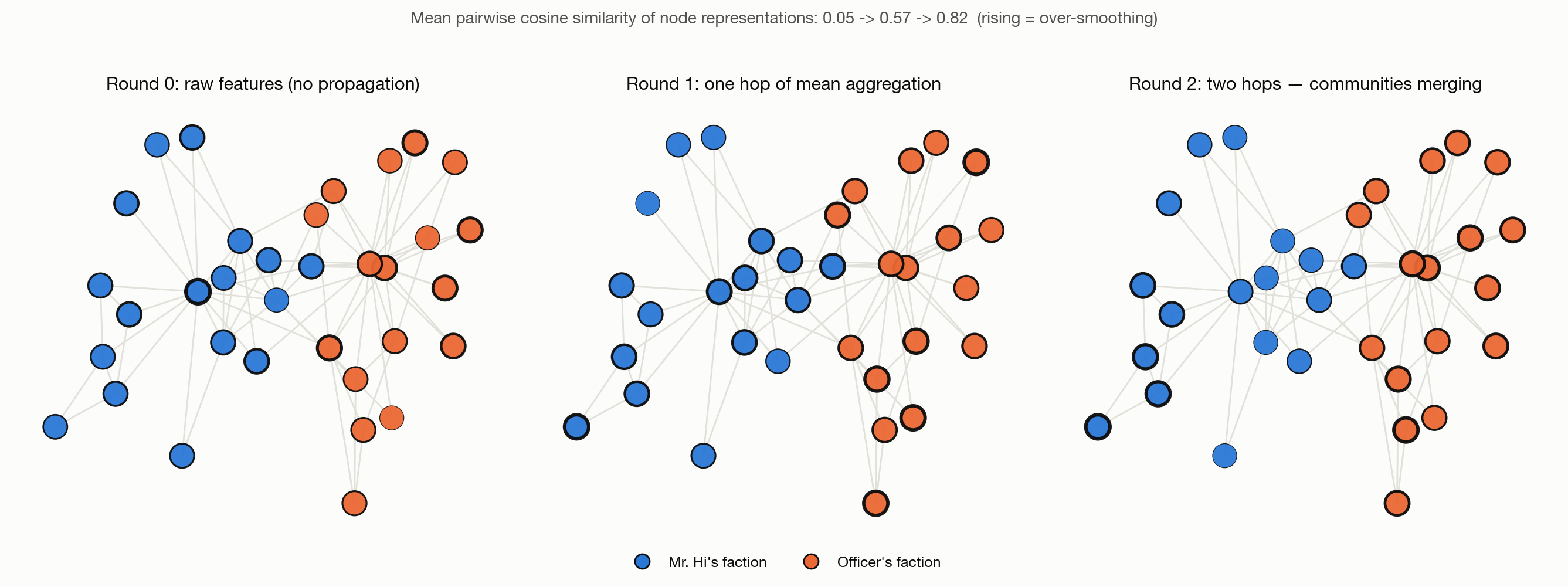
A distinctive failure mode of GNNs, absent (or at least much milder) in CNNs and RNNs, is over-smoothing: as \(K\) grows, node representations across the whole graph — not just within a neighborhood — converge toward each other and lose discriminative power. Depth is supposed to help (it grows the receptive field, letting distant information reach a node), but past a small number of layers it actively hurts, which is the opposite of the pattern in vision, where deeper networks (with residual connections) reliably help.
The intuition follows directly from the mean-aggregation update. Repeatedly averaging a node’s representation with its neighbors’ is, in matrix form, repeated multiplication by a (row-normalized) adjacency-derived operator: \(H^{(k)} = \hat{A} H^{(k-1)}\), where \(\hat{A}\) is the adjacency matrix with self-loops, row-normalized to be a stochastic matrix. This is precisely the transition matrix of a random walk on the graph. Repeated multiplication by a stochastic matrix is exactly what computes the stationary distribution of a random walk — and for a connected, non-bipartite graph that stationary distribution is unique and shared by every node, regardless of where the walk started. As \(K \to \infty\), \(H^{(k)}\) converges toward a matrix in which every row is proportional to the same vector (weighted by the graph’s degree structure): every node’s representation becomes an (almost) identical smoothed average over the whole connected component. Formally, this is the same convergence-to-stationary-distribution argument used for Markov chains in the Sampling and Approximate Inference chapter, applied here to features rather than to samples.
The practical consequence: 2-3 layers is the typical sweet spot for most GNN benchmarks. Beyond that, accuracy on node-classification tasks tends to drop, not because the model is overfitting but because the representations literally stop carrying useful, node-specific signal. Section 3 of the figure below shows this directly on a small graph: mean pairwise cosine similarity between node representations rises sharply after just two rounds of propagation. Mitigations exist — residual/skip connections that let a layer retain its pre-aggregation state, PairNorm and other normalization schemes that explicitly re-separate representations, “jumping knowledge” architectures that concatenate representations from every layer rather than just the last — but they manage the symptom rather than eliminate the underlying convergence behavior of iterated local averaging.
11.2 Main methods
GCN — Graph Convolutional Network
The Graph Convolutional Network (Kipf & Welling, 2017) is the simplest and most-cited instantiation of the message-passing template. Its aggregation is a fixed, symmetric-normalized mean over neighbors (including a self-loop):
\[ H^{(k)} = \sigma\!\left(\hat{D}^{-1/2} \hat{A} \hat{D}^{-1/2} H^{(k-1)} W^{(k)}\right) \]
where \(\hat{A} = A + I\) adds self-loops and \(\hat{D}\) is its degree matrix. The symmetric normalization (rather than plain row-normalization) keeps the propagation numerically well-behaved regardless of degree skew and has a spectral-graph-theory derivation as a first-order approximation of spectral convolutions on graphs — but in practice it’s usually simplest to think of it as “each node’s new representation is close to the (degree-weighted) average of its neighbors’ representations, linearly transformed.” GCN is transductive in its original formulation: it operates on the full, fixed adjacency matrix of one graph, and doesn’t natively generalize to unseen nodes or a different graph at inference time. It’s a strong, low-parameter baseline, but its uniform, un-weighted neighbor averaging throws away information about which neighbors matter more, and its transductive nature is a real limitation in production settings where new nodes (new users, new items, new molecules) appear after training.
GAT — Graph Attention Network
The Graph Attention Network replaces GCN’s fixed averaging with learned, content-dependent attention weights over neighbors — directly analogous to how self-attention in a Transformer (see Deep Learning Foundations) replaces a fixed convolution with query/key-driven weighting. For node \(v\) and each neighbor \(u \in \mathcal{N}(v)\), GAT computes an unnormalized attention score from both nodes’ current features, typically
\[ e_{vu} = \text{LeakyReLU}\!\left(a^\top [W h_v \,\|\, W h_u]\right) \]
then normalizes with softmax over \(v\)’s neighborhood to get \(\alpha_{vu}\), and aggregates as \(h_v^{(k)} = \sigma\left(\sum_{u \in \mathcal{N}(v)} \alpha_{vu} W h_u\right)\). Multi-head attention (running several independent attention mechanisms in parallel and concatenating or averaging their outputs) is standard, for the same variance-reduction and representational-diversity reasons it’s standard in Transformers. The payoff is that GAT can learn that some neighbors matter far more than others for a given node — a fraud ring’s central hub node shouldn’t be represented identically to a hub that’s just well-connected — without hand-designing edge weights. The cost is more parameters and compute per layer, and, like GCN in its base form, it’s typically applied transductively, though it’s easier to adapt to new nodes than GCN because the attention mechanism doesn’t depend on a fixed global adjacency structure the way GCN’s normalized Laplacian does.
GraphSAGE — inductive representation learning via sampling
GraphSAGE (Hamilton, Ying & Leskovec, 2017) was designed explicitly to solve the problem GCN doesn’t: inductive learning on graphs that grow or change, including graphs at a scale where materializing the full adjacency matrix per layer is infeasible. Two ideas make this work:
- Learn an aggregator function, not a fixed set of per-node embeddings. Instead of learning a lookup table of node representations (as a transductive method effectively does), GraphSAGE learns aggregation and transformation functions that take any node’s neighbor features as input and produce a representation — so the same trained model can embed a node that didn’t exist during training, provided its features and local neighborhood are available.
- Sample, don’t enumerate, neighborhoods. A high-degree node (a celebrity account, a popular product) can have millions of neighbors; aggregating over all of them at every layer is both computationally infeasible and not particularly informative beyond a certain neighborhood size. GraphSAGE fixes a sample size per layer (e.g. sample up to 25 neighbors at layer 1, up to 10 at layer 2) and aggregates over that random subsample rather than the full neighbor set. This bounds the per-node computation and, crucially, bounds the total nodes touched by a \(K\)-layer forward pass to a fixed fan-out (\(25 \times 10\), not the true degree product), which is what makes GraphSAGE practical on graphs with billions of edges.
GraphSAGE’s aggregator can be mean, LSTM (applied over a random permutation of sampled neighbors — a slightly awkward fit, since LSTMs aren’t naturally permutation-invariant, but effective in practice), or max-pooling over a per-neighbor MLP. In production recommender and social-graph systems (this is essentially the architecture behind Pinterest’s PinSage and similar systems), sampling-based inductive GNNs like GraphSAGE are close to the default choice specifically because full-graph, transductive methods don’t scale and can’t handle the constant stream of new users and items.
Beyond these three
GCN, GAT, and GraphSAGE cover the core design axes (fixed vs. learned aggregation weights, transductive vs. inductive, full-neighborhood vs. sampled), but the space is much larger. Message-Passing Neural Networks (MPNNs) generalize the template to explicitly incorporate edge features, which matters for molecules (bond type, bond length) and is the standard formulation in computational chemistry. Graph Isomorphism Networks (GIN) use sum aggregation specifically because it’s the most expressive permutation-invariant aggregator with respect to distinguishing non-isomorphic graph structures — mean and max aggregation both provably lose some structural information that sum preserves, connecting directly to the theoretical question of what a GNN can and can’t distinguish (bounded, in the worst case, by the Weisfeiler-Leman graph isomorphism test). Graph Transformers drop locality-restricted message passing altogether and let every node attend to every other node, using the graph structure as a bias term (e.g. via positional encodings derived from the graph Laplacian) rather than a hard constraint on who can talk to whom — trading the inductive bias and scalability of local message passing for the flexibility that made Transformers dominant in text and vision.
11.3 When to use it / what can go wrong
When a GNN earns its complexity. The signal that matters is genuinely relational — a node’s label depends on its neighbors’ features or labels in a way that isn’t already captured by hand-built aggregate features. Molecule property prediction is the clean case: molecular activity is a function of atomic structure and bonding, not just a bag of atom counts. Fraud and anomaly detection on transaction or account graphs is another: a fraud ring is defined by how accounts connect to each other (shared devices, shared payment methods, dense unusual subgraphs), not by any single account’s standalone features. Knowledge graphs, citation networks, and traffic/road networks share the same property — the topology carries information a row-wise model structurally cannot see.
When it doesn’t. If the graph is sparse, close to a tree, or the useful signal is dominated by node-level features with only weak neighbor dependence, a well-engineered gradient-boosted tree on hand-crafted graph statistics (degree, PageRank, clustering coefficient, number of neighbors of each label, k-core number) will often match or beat a GNN at a fraction of the engineering and serving cost — this is a direct instance of the general tabular-data lesson from Trees, Ensembles, and Tabular ML: if the problem doesn’t need learned representations, don’t pay for them. GNNs also need enough structure and label density to learn from; on a graph that’s almost entirely disconnected components of size 1-2, message passing has nothing to aggregate and degenerates toward a per-node model with extra overhead.
Over-smoothing. As covered above, more layers eventually erases the very information the model was built to preserve. In practice this means depth is not a free knob the way it often is (with residual connections) in vision or language models — most successful GNNs are 2-4 layers deep, and going deeper requires explicit countermeasures (residual/skip connections, PairNorm, DropEdge, jumping-knowledge aggregation across layers) rather than just adding capacity.
Scalability on huge graphs. Real production graphs (a social network, a web graph, a large knowledge base) can have billions of nodes and edges. Full-batch training — computing a forward pass over the entire adjacency matrix at once — doesn’t fit in memory past a fairly modest graph size. Neighbor sampling (GraphSAGE-style), graph partitioning/clustering methods that train on manageable subgraphs (e.g. Cluster-GCN), and precomputing fixed diffusion/propagation matrices offline (so inference doesn’t require live graph traversal) are all standard responses, each trading off some approximation quality for tractability. A related, easy-to-miss issue is neighborhood explosion: without sampling, the number of nodes touched by a \(K\)-layer forward pass grows with the product of per-layer degrees, so even a moderate average degree can make \(K=3\) touch a large fraction of the graph for a single node’s prediction.
Feature and label leakage across edges. Because a node’s prediction literally depends on its neighbors’ features (and sometimes labels, in label-propagation-flavored setups), it’s easy to accidentally leak train/test information across the graph — a training node might have a test node as a direct neighbor, so its representation partially encodes the very label being held out for evaluation. Graph-aware splitting (holding out whole connected components or using temporal cutoffs, rather than a random per-node split) is necessary to get an honest estimate of generalization, and this bites practitioners often enough that it’s worth checking explicitly whenever a GNN benchmark result looks unusually strong.
Directionality and heterogeneity. Real graphs are often directed (a follows relationship, a citation) and heterogeneous (users, items, and categories are different node types with different feature spaces, connected by different edge types with different semantics). Applying a homogeneous, undirected message-passing scheme to a graph that’s neither can silently discard information a domain-appropriate architecture (relational GCNs, heterogeneous graph transformers, or simply separate weight matrices per edge type) would have used.
11.4 How this connects
- Representation Learning — a GNN is best understood as a representation-learning method whose inductive bias is “a node’s representation should be a function of its local neighborhood,” the same way a CNN’s inductive bias is spatial locality and a Transformer’s is pairwise attention; the embeddings a GNN produces feed downstream tasks exactly like any other learned representation.
- Sequence, Time-Series, and State Models — GAT’s attention mechanism is the same query/key/value idea used by self-attention in sequence models, applied over a node’s graph neighbors instead of over positions in a sequence; and the over-smoothing argument above (repeated stochastic-matrix multiplication converging to a stationary distribution) is the same Markov-chain convergence logic used to describe stationary behavior of recurrent state updates.
- Sampling and Approximate Inference — the random-walk view of mean aggregation ties GNN over-smoothing directly to Markov chain stationary distributions and mixing, the same machinery that underlies MCMC convergence.
- Information Retrieval, Ranking, and Recommenders — large-scale recommender and search systems increasingly use GNNs (e.g. GraphSAGE-style inductive embeddings) for candidate generation over a user-item interaction graph, treating retrieval itself as a graph-traversal and embedding-similarity problem rather than a purely tabular one.
- ML Systems and MLOps — serving GNN-based predictions in production surfaces graph-specific systems problems (feature stores that must serve live neighborhood lookups, sampling infrastructure for training on graphs too large to fit in memory) that don’t arise for row-independent tabular models.