5 Laplace Noise, Robustness, and Huber
Chapter 4 ended on a specific weakness: squared error’s quadratic growth lets a single large residual dominate the objective. This chapter asks the natural next question twice — once as a clean likelihood derivation, and once as a deliberate engineering compromise — because the two losses that answer it, MAE and Huber, come from genuinely different places, and conflating them would blur exactly the distinction this book insists on.
5.1 The problem
Same setup as Chapter 4: predict a real-valued \(y\) from \(x\). But now the noise around the true value is suspected to produce occasional large deviations more often than a Gaussian would predict — heavier tails — and a single contaminated or mismeasured point shouldn’t be allowed to swing the fit as far as Figure 4.1’s quadratic penalty allows it to.
5.2 Assumptions
\[ Y \mid X=x \;\sim\; \mathrm{Laplace}\big(f_\theta(x), b\big), \qquad p(y\mid x;\theta) = \frac{1}{2b}\exp\!\left(-\frac{|y-f_\theta(x)|}{b}\right). \]
The Laplace distribution is symmetric like the Gaussian, but its density decays linearly in log-space rather than quadratically — its tails are heavier, so it assigns meaningfully more probability to large deviations. Assuming Laplace noise is assuming that large errors, while still rare, aren’t as rare as a Gaussian would insist.
5.3 Derivation
From Laplace likelihood to MAE
Following the identical pattern as Chapter 4:
\[ -\log p(y\mid x;\theta) = \frac{|y-f_\theta(x)|}{b} + \log(2b). \]
\(\log(2b)\) doesn’t depend on \(\theta\); \(1/b\) is a positive constant that rescales but doesn’t relocate the minimum. So
\[ \mathrm{NLL}(\theta) \propto \sum_{i=1}^n |y_i - f_\theta(x_i)| \]
— mean absolute error, exactly, by the same likelihood machinery as Chapter 4, with Laplace in place of Gaussian.
What MAE’s minimizer actually is
\(\arg\min_a \mathbb{E}|Y-a|\) is a median of \(Y\), not its mean. A short argument: the subgradient of \(|Y-a|\) with respect to \(a\) is \(-1\) where \(a<Y\) and \(+1\) where \(a>Y\), so \(\frac{d}{da}\mathbb{E}|Y-a| = P(Y<a) - P(Y>a)\); setting this to zero gives \(P(Y<a)=P(Y>a)\), the defining property of a median. Applied pointwise, \(\arg\min f_\theta(x)\) under expected absolute error is a conditional median of \(Y\mid X=x\), not a conditional mean — a second, independent confirmation of Chapter 1’s claim that different losses want fundamentally different predictions. (The median’s well-known insensitivity to how far outliers sit — a point can move arbitrarily far away without changing which point is “in the middle” — is the population-level reason MAE resists outliers where MSE doesn’t.)
Huber, pseudo-Huber, and log-cosh: designed compromises
MAE fixes the outlier problem but introduces one of its own: a constant- magnitude gradient everywhere except a kink at exactly zero residual, which never shrinks as a fit gets close to correct — a real complication for gradient-based optimization, developed in the next section. Huber’s loss (Huber 1964) is built explicitly to fix both problems at once: quadratic (and so smoothly, shrinking-gradient) near zero, linear (and so outlier-resistant) far from it —
\[ \ell_\delta(r) = \begin{cases} \tfrac{1}{2}r^2 & |r| \le \delta \\ \delta\left(|r| - \tfrac{1}{2}\delta\right) & |r| > \delta \end{cases}, \qquad r = y - f_\theta(x). \]
Pseudo-Huber (\(\delta^2(\sqrt{1+(r/\delta)^2}-1)\)) and log-cosh (\(\delta^2\log\cosh(r/\delta)\)) are smoother variants with the same qualitative near-zero-quadratic, far-away-linear shape, trading an exact kink for full differentiability everywhere at the cost of a slightly more expensive formula.
5.4 The resulting objectives
\[ \ell_{\mathrm{MAE}}(\theta;x,y) = |y - f_\theta(x)| \]
Exactly as direct a consequence of the Laplace assumption as MSE is of the Gaussian one in Chapter 4 — not a heuristic robustness fix, even though it happens to behave more robustly.
\[ \ell_\delta(\theta;x,y) = \begin{cases} \tfrac{1}{2}(y-f_\theta(x))^2 & |y-f_\theta(x)| \le \delta \\ \delta\big(|y-f_\theta(x)| - \tfrac{1}{2}\delta\big) & \text{otherwise} \end{cases} \]
Huber is not simply invented. It is the exact NLL of a legitimate (if unusual) noise density built by gluing a Gaussian center to Laplace tails at \(\pm\delta\) — so a likelihood reading genuinely exists. But that is not why Huber is used in practice: it’s used because of the gradient behavior derived below, chosen by picking \(\delta\) to trade off robustness against convergence speed rather than by asserting a belief about the true noise distribution. Call it hybrid: a real likelihood interpretation is available, but the reason for reaching for it is almost always optimization behavior, not a statistical belief about the data-generating process.
5.5 Interpretation
MAE’s minimizer is a conditional median, as derived above — robust to how far an outlier sits, only sensitive to which side of it points fall on. Huber interpolates: for residuals inside \(\pm\delta\) it behaves exactly like squared error (pulling toward something mean-like), and for residuals outside \(\pm\delta\) it behaves exactly like absolute error (pulling toward something median-like) — its minimizer isn’t a single named statistic of \(Y\mid X=x\) in general, which is itself informative: chasing “a clean statistical interpretation” and “good optimization behavior” can pull in different directions, and Huber openly picks a point between them rather than resolving the tension.
5.6 Behavior and edge cases
Figure 5.1 plots loss and gradient together for all three. MSE’s gradient is unbounded — a residual of 10 produces ten times the gradient of a residual of 1, actively amplifying the influence of whatever produced that residual, outlier or not. MAE’s gradient has constant magnitude 1 everywhere except a discontinuity exactly at \(r=0\), where the loss is non-differentiable — this makes plain gradient descent oscillate right at the optimum rather than settle into it smoothly. Huber matches MSE’s smooth, shrinking gradient near zero and MAE’s bounded gradient far away, with no discontinuity anywhere.
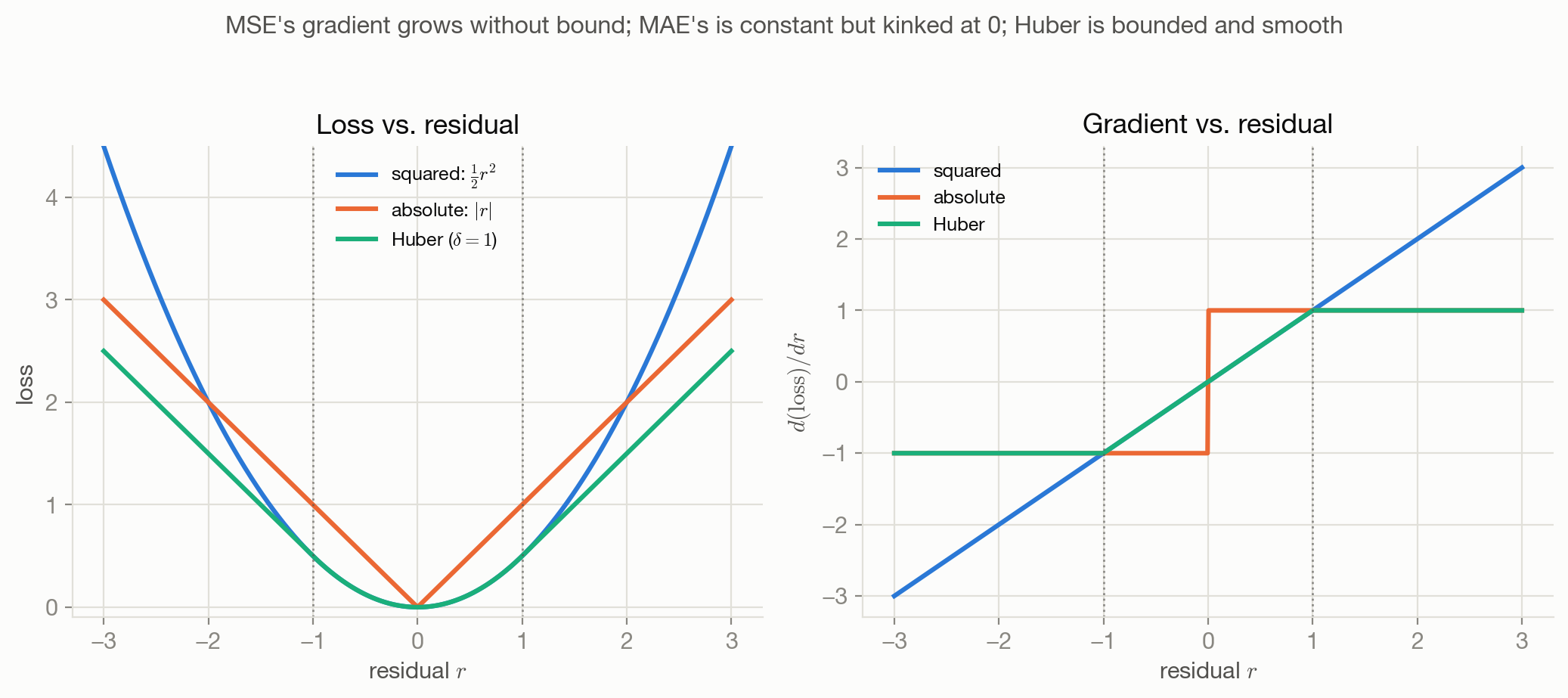
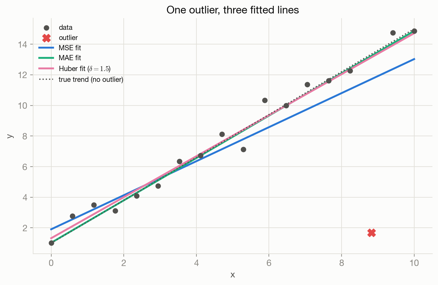
Figure 5.2 makes the practical consequence concrete on a real (if small) fit: eighteen points on a line, one deliberately corrupted far below the trend. The MSE-fit line is visibly dragged toward the outlier; the MAE and Huber fits stay close to the true trend, barely perturbed.
5.7 Limitations
MAE’s robustness is a double-edged property: it’s exactly as unmoved by a single catastrophic outlier as it is by a single point that’s meaningfully, but not enormously, off — it doesn’t distinguish “slightly wrong” from “very wrong” beyond the sign of the residual dictating gradient direction, which can be too coarse when moderate errors should still matter more than tiny ones. Huber’s compromise depends on choosing \(\delta\) well: too small and it behaves like MAE everywhere that matters; too large and it behaves like MSE everywhere that matters, in both cases forfeiting the reason to use it at all.
5.8 Optimization implications
MAE’s gradient discontinuity at \(r=0\) means subgradient methods (or a smoothed surrogate, as used for fig_outlier_robustness.py’s numerical fit) are needed for a fully rigorous treatment, and plain gradient descent tends to oscillate near the optimum rather than converge smoothly into it. Huber was designed in significant part to avoid exactly this — see Chapter 17 for a direct three-way optimization comparison once surrogate losses (Chapter 9) are also on the table.
5.9 Connections
- Chapter 4 is this chapter’s direct counterpart and the source of the outlier-sensitivity problem this chapter addresses.
- Chapter 3 uses the Laplace distribution in its other role, as a prior over \(\theta\) producing \(\ell_1\)/Lasso regularization — a genuinely different construction from this chapter’s use of Laplace as a likelihood over \(y\).
- Chapter 8 derives the median-minimizer result above from decision theory directly, without needing a Laplace likelihood at all.
- Chapter 9 continues the robustness-vs- optimization-tradeoff theme into classification, where hinge and logistic loss make a structurally similar compromise for a different reason.