4 Gaussian Noise and Squared Error
Squared error is usually the very first loss anyone meets, often introduced by fiat: predictions should be close to targets, and squaring a residual is a convenient way to make “close” a differentiable, always-positive number. That story isn’t wrong, exactly, but it skips the more interesting fact. Squared error is not a convenient invention — it is the exact negative log-likelihood of one specific, nameable assumption about how a target is generated. Chapter 2 built the machine that turns a probabilistic assumption into a loss; this chapter is the machine’s first real output.
4.1 The problem
A regression problem asks for a function \(f_\theta(x)\) that predicts a real-valued target \(y\). Chapter 2 reframed “predicts” probabilistically: instead of \(f_\theta\) outputting a bare number, it parameterizes a full conditional distribution \(p(y\mid x;\theta)\), and NLL under that distribution becomes the loss. What distribution is appropriate when a target is a real number corrupted by some kind of measurement or process noise around a “true” value \(f_\theta(x)\)?
4.2 Assumptions
\[ Y \mid X = x \;\sim\; \mathcal{N}\big(f_\theta(x),\, \sigma^2\big), \]
with the noise i.i.d. across examples and, for now, a single fixed \(\sigma^2\) shared by every \(x\) (homoscedastic noise). This says: the target is the model’s prediction plus symmetric, bell-shaped noise of a fixed spread — no systematic skew, no outlier-prone heavy tails, and critically, a spread that doesn’t depend on \(x\). Each of these is a real assumption, not a fact, and each has consequences worked out below and in Chapter 5.
4.3 Derivation
Fixed-variance case
The Gaussian density is \(p(y\mid x;\theta) = \frac{1}{\sqrt{2\pi\sigma^2}} \exp\!\left(-\frac{(y-f_\theta(x))^2}{2\sigma^2}\right)\). Its negative log is
\[ -\log p(y\mid x;\theta) = \frac{(y-f_\theta(x))^2}{2\sigma^2} + \frac{1}{2}\log(2\pi\sigma^2). \]
The second term doesn’t involve \(\theta\) at all — \(\sigma^2\) is fixed and \(2\pi\) is a constant — so it drops out of any \(\arg\min_\theta\). Summed over a dataset, using the notation from Chapter 2:
\[ \mathrm{NLL}(\theta) = \sum_{i=1}^n \left[\frac{(y_i-f_\theta(x_i))^2}{2\sigma^2}\right] + \text{const} \;\propto\; \sum_{i=1}^n (y_i - f_\theta(x_i))^2. \]
Minimizing NLL under this assumption is, exactly and not just approximately, minimizing sum of squared errors — the constant \(1/(2\sigma^2)\) only rescales the objective and does not move its minimizer. This is worth sitting with: the humble MSE loss used everywhere is the Gaussian NLL, full stop, not “sort of like” it.
What the assumed noise level controls
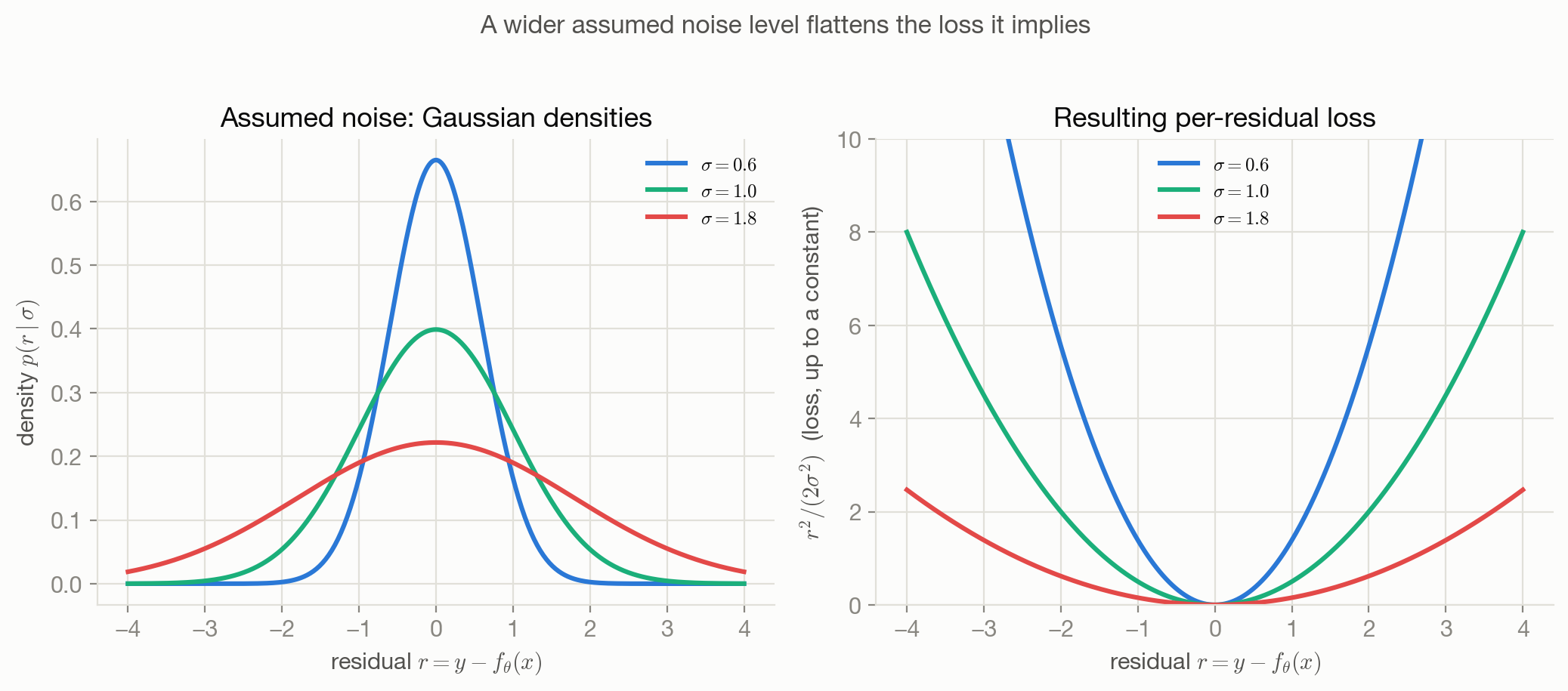
Even though \(\sigma^2\) doesn’t affect where the fixed-variance NLL is minimized, it does control the loss’s shape: the loss is \(\frac{r^2}{2\sigma^2}\) as a function of the residual \(r = y - f_\theta(x)\), so a larger assumed \(\sigma^2\) produces a flatter parabola — every residual is penalized less. Figure 4.1 shows this directly: three assumed noise levels, their corresponding Gaussian densities, and the per-residual loss curve each one implies. A model told “I expect noise with \(\sigma=1.8\)” is being told, in the same breath, “don’t work too hard to close a residual of size 2” — assuming more noise and discounting errors more heavily are the same statement.
Heteroscedastic regression: when noise itself depends on \(x\)
The fixed-\(\sigma^2\) assumption is often wrong: measurement noise on a sensor can scale with the reading, forecast uncertainty can be genuinely larger for some inputs than others. Let the model output a per-input variance too, \(\sigma_\theta(x)^2\), so \(Y\mid X=x \sim \mathcal{N}(f_\theta(x), \sigma_\theta(x)^2)\). Repeating the derivation above, but now keeping the variance term because it depends on \(\theta\) through \(x\):
\[ \mathrm{NLL}(\theta) = \sum_{i=1}^n\left[\frac{(y_i - f_\theta(x_i))^2}{2\sigma_\theta(x_i)^2} + \frac{1}{2}\log\sigma_\theta(x_i)^2\right] + \text{const}. \]
This is a genuinely different objective from plain MSE, not a rescaled copy of it. The first term is a squared error weighted by \(1/\sigma_\theta(x)^2\): points the model claims to be uncertain about matter less to the loss. The second term is what stops the model from gaming this — claiming huge uncertainty everywhere would shrink the first term toward zero for free, but \(\frac{1}{2}\log\sigma_\theta(x)^2\) grows (less negative reward) as claimed variance grows, penalizing overconfident claims of uncertainty just as much as overconfident predictions. The two terms together force the model to predict a variance that’s actually calibrated to where it tends to be wrong.
4.4 The resulting objective
\[ \ell_{\mathrm{MSE}}(\theta; x, y) = (y - f_\theta(x))^2, \qquad \hat R(\theta) = \frac{1}{n}\sum_{i=1}^n (y_i - f_\theta(x_i))^2. \]
Fixed-variance MSE is the Gaussian NLL with the variance term dropped as a constant — a direct consequence of assuming symmetric, constant-spread noise, not a design choice made for convenience. The heteroscedastic variant above is the same likelihood-derived origin, just without dropping the now-informative variance term.
4.5 Interpretation
Minimizing expected squared error \(\mathbb{E}[(Y-a)^2]\) over a constant \(a\) is minimized at \(a = \mathbb{E}[Y]\) — the conditional mean. (Differentiate and set to zero: \(-2\mathbb{E}[Y-a]=0 \Rightarrow a = \mathbb{E}[Y]\).) Applied pointwise at every \(x\), this means the population-optimal \(f_\theta(x)\) under squared error is \(\mathbb{E}[Y\mid X=x]\) — squared error’s minimizer is defined to be the conditional mean, regardless of what the true conditional distribution of \(Y\) actually looks like. Chapter 8 proves this in general, via decision theory rather than calculus, and shows exactly why other losses recover other statistics of \(Y\mid X=x\).
4.6 Behavior and edge cases
Quadratic growth means a residual twice as large costs four times as much, not twice as much — the loss actively prioritizes fixing the single worst prediction over many small ones. That’s desirable when big errors really are disproportionately bad; it’s a liability when a few contaminated or mismeasured points shouldn’t be allowed to dominate the fit. A single outlier can pull \(f_\theta\) noticeably away from where it would sit for the bulk of well-behaved data — precisely the failure mode Chapter 5 is built to address, and demonstrates concretely on a synthetic dataset.
4.7 Limitations
Everything above only holds insofar as the Gaussian assumption is approximately right. Heavy-tailed noise (occasional large errors far more common than a Gaussian would predict) makes the fixed-variance MSE fit overly sensitive to exactly those rare large errors, since they’re precisely what a squared penalty punishes hardest. Skewed noise makes “symmetric penalty around the mean” the wrong target altogether. And the heteroscedastic extension only helps if \(\sigma_\theta(x)\) is itself well-specified — a badly-fit variance model can miscalibrate the weighting term above just as easily as it can correctly calibrate it.
4.8 Optimization implications
Squared error is smooth and strictly convex in \(f_\theta(x)\) for every fixed \(x\), with a gradient that’s linear in the residual (\(\partial \ell/\partial f_\theta(x) = -2(y-f_\theta(x))\)) — well-behaved near the optimum, but also unbounded far from it, so a single very wrong prediction contributes a very large gradient. For a linear \(f_\theta\), this is the ordinary least-squares problem with the closed-form, well-conditioned solution machinery of optimization-lab. Chapter 17 compares this gradient behavior directly against MAE’s and Huber’s.
4.9 Connections
- Chapter 1 and Chapter 2 supply, respectively, the general notion of a loss and the NLL machine this chapter is the first concrete output of.
- Chapter 3 uses a Gaussian in a different role — as a prior over \(\theta\), producing \(\ell_2\) regularization, not as a likelihood over \(y\). Worth holding both uses in mind at once; they’re easy to conflate.
- Chapter 5 swaps the Gaussian for a Laplace assumption and derives MAE, with a direct outlier-robustness comparison against this chapter’s MSE.
- Chapter 8 proves the conditional-mean interpretation above from decision theory, independent of any distributional assumption.