12 Reinforcement Learning and Bandits
Every method covered so far learns from a fixed dataset of examples that already exist. Reinforcement learning (RL) is different in kind: it studies an agent that takes actions inside an environment, receives a reward signal for each action, and — critically — whose actions change what happens next. There is no dataset handed over in advance; the agent has to generate its own experience by acting, observe the consequences, and use that experience to get better at choosing actions. This is the right framing whenever a decision today affects the situation you’ll face tomorrow: playing a game, routing a robot, managing inventory, sequencing a conversation with a user, or choosing which arm of a slot machine to pull. Bandits are the simplified special case of this problem where actions do not affect future state — every round looks the same regardless of what happened before — which strips away the hardest part of RL (long-horizon credit assignment) and leaves a purer version of the other hard part: balancing exploration against exploitation under uncertainty.
12.1 How it works
The Markov Decision Process
The standard formalization of the full RL problem is a Markov Decision Process (MDP): a tuple of states \(\mathcal{S}\), actions \(\mathcal{A}\), a transition function \(P(s' \mid s, a)\) giving the probability of landing in state \(s'\) after taking action \(a\) in state \(s\), a reward function \(R(s, a, s')\), and a discount factor \(\gamma \in [0, 1)\). An agent’s behavior is a policy \(\pi(a \mid s)\), a mapping from states to a distribution over actions. The goal is to find a policy that maximizes expected cumulative discounted reward, \(\mathbb{E}\left[\sum_{t=0}^{\infty} \gamma^t R_t\right]\).
The “Markov” in MDP is doing real work: it asserts that \(P(s' \mid s, a)\) depends only on the current state and action, not on the full history that led there. This is the same conditional-independence assumption that defines a hidden Markov model in the Graphical Models and Latent Variables chapter, applied here to a controlled process rather than a passively-observed one — the state is defined precisely to be “whatever summary of history is sufficient to predict the future,” which is why so much of applied RL engineering is really about state design: choosing a representation rich enough that the Markov property actually holds (or holds closely enough).
The discount factor \(\gamma\) matters for reasons beyond “reward now is better than reward later.” It makes infinite-horizon returns finite and well-defined whenever rewards are bounded, and mathematically it also determines how strongly the value of a state depends on distant future rewards — small \(\gamma\) produces myopic, short-horizon behavior; \(\gamma\) close to 1 forces the agent to reason many steps ahead, which is both more powerful and much harder to estimate accurately from limited experience.
Value functions and the Bellman equation
The central objects RL algorithms compute are value functions: the state value \(V^\pi(s) = \mathbb{E}_\pi\left[\sum_t \gamma^t R_t \mid s_0 = s\right]\), the expected return starting from \(s\) and following policy \(\pi\) thereafter, and the action value \(Q^\pi(s, a)\), the same quantity but conditioned on taking action \(a\) first. These satisfy a recursive consistency condition called the Bellman equation:
\[ V^\pi(s) = \sum_a \pi(a \mid s) \sum_{s'} P(s' \mid s, a) \big[R(s, a, s') + \gamma V^\pi(s')\big] \]
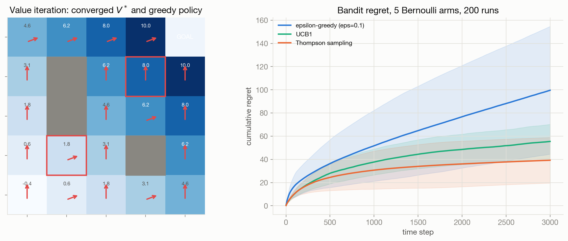
This says something almost tautological but extremely useful: the value of a state equals the immediate expected reward plus the discounted value of wherever you land next. It’s a fixed-point equation — \(V^\pi\) is the function that, when you plug it into the right-hand side, reproduces itself. This matters because it turns “find the value function” from a search problem into a fixed-point problem, which comes with a ready-made solution method: iterate the update repeatedly and it will converge, by the Banach fixed-point theorem, because the Bellman operator is a contraction under the \(\gamma < 1\) discount (each application of the operator shrinks the worst-case error to the true value function by a factor of \(\gamma\)). This is exactly what value iteration does: start with an arbitrary \(V\), repeatedly apply \(V(s) \leftarrow \max_a \sum_{s'} P(s' \mid s, a)[R + \gamma V(s')]\) for every state (replacing the policy-weighted sum with a max, since the optimal value function satisfies the Bellman optimality equation, not just consistency under a fixed policy), and stop once \(V\) stops changing meaningfully. Figure 12.1 (left) shows exactly this run to convergence on a small gridworld: the heatmap is the converged \(V^*\), and the arrows show the greedy policy — the action that maximizes the one-step Bellman backup at each cell — reading off directly from those values.
Once you have \(Q^\pi\), extracting a good policy is simple: act greedily, \(\pi(s) = \arg\max_a Q(s, a)\). This is the mechanism behind essentially every value-based RL method — the hard part isn’t turning values into a policy, it’s estimating accurate values in the first place, especially when \(P\) and \(R\) aren’t known in advance and have to be estimated from the agent’s own experience.
The exploration-exploitation tradeoff
An agent that only ever exploits — always picks the action that currently looks best — can get permanently stuck on a mediocre action it happened to try early and never discover a better one, because it never generates the data that would reveal the better option. An agent that only ever explores never capitalizes on what it has learned. Every RL and bandit algorithm has to resolve this tension somehow, and the specific mechanism it uses is the main thing that distinguishes one algorithm from another.
12.2 Main methods
Bandits: exploration-exploitation without state
In the multi-armed bandit setting, there is one state (or none, meaningfully), \(K\) actions (“arms”), and each arm produces reward from a fixed but unknown distribution. There is no long-term consequence to pulling an arm beyond the immediate reward — so the entire problem reduces to estimating each arm’s expected reward accurately enough, quickly enough, to stop wasting pulls on worse arms. Contextual bandits add side information (a context vector, e.g. features of the user being served) that the reward distribution depends on, turning the problem into learning a mapping from context to best-action-in-context rather than a single global ranking of arms — this is the standard formulation for ad selection, article/content recommendation, and notification targeting, where “arm” is a candidate item and “context” is the user and situation.
Three canonical strategies, each trading off exploration differently:
- Epsilon-greedy. With probability \(\epsilon\), pick a uniformly random arm; otherwise pick the current best estimate. Simple, and it never converges to zero exploration unless \(\epsilon\) is explicitly decayed — which means it keeps paying a constant per-round exploration cost forever, even long after it has enough data to know which arm is best. This shows up directly in Figure 12.1 (right): epsilon-greedy’s regret grows roughly linearly because a fixed fraction of pulls are wasted at every time step, no matter how much has already been learned.
- UCB (Upper Confidence Bound). Instead of picking the arm with the highest estimated mean, pick the arm with the highest estimated mean plus an uncertainty bonus that shrinks as that arm is pulled more: \(\arg\max_a \hat{\mu}_a + c\sqrt{\ln t / n_a}\). This is “optimism in the face of uncertainty” — arms that haven’t been tried much get an inflated score precisely because their estimate is unreliable, which automatically directs exploration toward arms that are either promising or under-tested, and lets it taper off (in expectation, logarithmically) as evidence accumulates. UCB1’s regret bound is \(O(\log T)\), provably better than fixed epsilon-greedy’s \(O(T)\) asymptotically, which is exactly the crossover visible in the right panel of the figure.
- Thompson sampling. Maintain a posterior distribution over each arm’s true reward rate (e.g. a Beta distribution for Bernoulli rewards, updated conjugately after every pull — the same conjugate-update machinery described in Probabilistic Modeling), and on each round, draw one sample from each arm’s posterior and act greedily with respect to the samples. Arms with wide, uncertain posteriors will occasionally sample a high value and get tried; arms that are confidently known to be bad will almost never win the draw. This is a fully Bayesian resolution of the exploration-exploitation tradeoff and tends to perform at least as well as UCB in practice while being simple to implement whenever a reasonable prior/likelihood pair is available.
Dynamic programming, Monte Carlo, and temporal difference learning
When the environment’s transition and reward functions are fully known, dynamic programming methods — value iteration and policy iteration — can compute the exact optimal value function and policy by repeated application of the Bellman equation, as described above. This is the easy case, and it’s rare in practice: usually the transition dynamics are unknown and can only be sampled by acting.
Monte Carlo methods estimate value functions purely from complete episodes: run the policy to termination, then update value estimates toward the actually-observed return. This is unbiased but high-variance (a single episode’s outcome can depend on a long chain of random events) and requires episodes to actually terminate, which rules out continuing tasks.
Temporal difference (TD) learning is the key idea that makes most modern RL practical: instead of waiting for the full episode to end, update the value estimate using the next reward plus the current estimate of the value of the next state — bootstrapping off its own current estimate rather than waiting for ground truth. The TD(0) update is \(V(s_t) \leftarrow V(s_t) + \alpha\big[R_t + \gamma V(s_{t+1}) - V(s_t)\big]\), where the bracketed term is the TD error: the gap between what the value function currently predicts and a one-step-better estimate of the truth. This trades some bias (bootstrapping off a possibly-wrong estimate) for dramatically lower variance and the ability to learn online, one step at a time, without waiting for episodes to finish — the same bias-variance tradeoff that shows up throughout Supervised Learning, here playing out across time rather than across model complexity.
Q-learning applies TD updates directly to the action-value function, and does so off-policy: it updates \(Q(s, a)\) using the best next action regardless of which action the exploration policy (e.g. epsilon-greedy) actually took — \(Q(s_t, a_t) \leftarrow Q(s_t, a_t) + \alpha\big[R_t + \gamma \max_{a'} Q(s_{t+1}, a') - Q(s_t, a_t)\big]\). This lets the same experience be used to learn about the optimal policy even while behaving exploratorily. SARSA is the on-policy sibling: it bootstraps using the value of the action the policy actually takes next (hence the name — state, action, reward, state, action), which makes it learn the value of the policy actually being followed, exploration noise included — a meaningfully different and often safer target when exploratory actions carry real risk, since SARSA’s estimates account for the chance of taking a bad exploratory action, while Q-learning’s optimistic max implicitly assumes you’ll always act optimally going forward.
Policy gradients and actor-critic methods
Value-based methods learn \(Q\) or \(V\) and derive a policy indirectly by acting greedily. Policy gradient methods instead parameterize the policy directly, \(\pi_\theta(a \mid s)\), and optimize its parameters via gradient ascent on expected return, using the policy gradient theorem to get an unbiased gradient estimate from sampled trajectories, \(\nabla_\theta J(\theta) = \mathbb{E}\big[\nabla_\theta \log \pi_\theta(a \mid s) \cdot G\big]\), where \(G\) is the observed return following that action. This has real advantages: it works naturally with continuous action spaces (where “take the argmax over actions” isn’t well-defined the way it is for a small discrete action set), and it can represent stochastic policies directly, which matters in partially-observed or adversarial settings where a deterministic policy is exploitable. The cost is high variance in the gradient estimate, since \(G\) depends on an entire sampled trajectory’s worth of randomness.
Actor-critic methods reduce that variance by learning both a policy (the “actor”) and a value function (the “critic”), using the critic’s value estimate as a baseline to subtract from the return — replacing raw \(G\) with an advantage estimate \(A(s, a) = Q(s,a) - V(s)\), which has the same expectation but much lower variance, since it measures “how much better than average was this action” rather than the raw, high-variance realized return. This actor-critic structure, scaled up with deep networks for both components, is the backbone of most modern policy-gradient RL, including the optimization step behind RLHF (below).
Offline RL
Offline RL (also called batch RL) learns a policy purely from a fixed, previously-logged dataset of interactions — no further exploration allowed. This matters enormously in practice: for a recommendation system, a medical treatment policy, or a robot, letting an under-trained agent explore live against real users, patients, or hardware is often unacceptable. The core difficulty is distributional shift: the learned policy’s value estimates are only reliable for state-action pairs the logging policy actually visited with reasonable frequency; anywhere the learned policy wants to deviate toward under-covered actions, its own value function is extrapolating into territory it has no real evidence about — and because Q-learning-style bootstrapping tends to be optimistically biased under extrapolation, offline RL without correction reliably overestimates the value of exactly those poorly-covered actions, encouraging the policy to drift toward exactly the gaps in the data. Effective offline RL methods (conservative Q-learning, behavior-regularized approaches) explicitly penalize the policy for deviating too far from what the logged behavior policy actually did, trading some potential improvement for reliability given only fixed data.
RLHF: RL as an alignment tool
Reinforcement learning from human feedback (RLHF) is the technique that turns human preference judgments into a training signal for large language models. The typical pipeline: collect pairs of model outputs, have humans (or a model trained to imitate them) indicate which is preferred; train a reward model to predict that preference (usually via a Bradley-Terry-style pairwise loss); then optimize the language model’s policy — token generation as sequential action selection — against that learned reward using a policy-gradient method (commonly PPO, an actor-critic method with a clipped objective for training stability), while penalizing large departures from a reference policy (usually via a KL penalty) to keep generations coherent and prevent reward-hacking exploits of an imperfect reward model. Structurally, this is exactly the RL problem: a policy (the language model), actions (tokens), and a reward signal — just one where the reward model itself was learned from data rather than specified by an engineer, which ties RLHF as much to the Causal Inference and Experimentation and evaluation problem of “does this proxy reward actually track what we want” as it does to RL mechanics per se.
12.3 When to use it / what can go wrong
When RL is the right framing. Use it when actions genuinely affect future state and the problem has real sequential structure — a game, a physical control problem, a multi-turn dialogue, a resource-allocation process that carries over time. Use a bandit specifically when actions do not meaningfully affect future context — ad selection, ranking exploration on a single request, notification timing — because the bandit formulation is simpler to reason about, faster to converge, and doesn’t require estimating anything about long-horizon dynamics that don’t actually exist in the problem.
When not to reach for RL. If supervised labels of “the right action” are directly available, use supervised learning — it’s more sample-efficient, easier to debug, and doesn’t carry the exploration risk. If the action really doesn’t affect future state, model it as a bandit, not a full MDP — trying to learn transition dynamics that don’t exist just adds variance for no benefit. If exploration is unsafe (a wrong action in a medical, financial, or physical system can cause real, irreversible harm), either use offline RL with conservative value estimation, restrict exploration to a simulator, or don’t use RL at all — a well-validated heuristic or supervised policy with human oversight is often the responsible choice even if it’s less theoretically optimal. And if the reward signal is poorly defined or easy to hack (a proxy metric that can be gamed without actually achieving the intended goal — e.g. “maximize watch time” as a stand-in for “recommend genuinely good content”), RL will find and exploit exactly that gap, often before anyone notices; reward design deserves as much scrutiny as the algorithm itself.
Common failure modes. Reward hacking — the agent finds a way to score well on the literal reward function that doesn’t match the designer’s actual intent — is close to a law of nature in RL and gets worse, not better, as optimization pressure increases. Sample inefficiency is a persistent practical problem: model-free deep RL often needs orders of magnitude more interaction data than a human would to learn a comparably good policy, which is part of why offline RL and simulation are so heavily used in practice. Non-stationary environments (a market, a set of competing agents, a user base whose preferences drift) break the fixed-MDP assumption outright and require either continual re-training or explicit non-stationarity handling. Off-policy value estimation from logged data (the same problem underlying offline RL) is easy to get subtly, silently wrong — it’s worth validating any offline value estimate against a genuine held-out interventional signal before trusting it operationally, in the same spirit as the causal-inference caution against trusting an unvalidated observational estimate.
12.4 How this connects
- Probabilistic Modeling — Thompson sampling is Bayesian inference applied directly to decision-making: the conjugate posterior updates that chapter develops for coin-flip-like data are exactly what drives arm selection here.
- Sampling and Approximate Inference — Monte Carlo return estimation is literally Monte Carlo estimation applied to trajectories, and the same variance-reduction motivations (importance sampling, baselines) that show up there recur in policy-gradient variance reduction here.
- Causal Inference and Experimentation — contextual bandits are, in a real sense, adaptive experiments: choosing which arm to show next based on accumulating evidence is exactly the problem multi-armed bandit designs address as an alternative to fixed A/B testing, and offline RL’s distributional-shift problem is a close cousin of confounding and positivity violations in observational causal inference.
- Information Retrieval, Ranking, and Recommenders — bandits are the standard tool for ranking exploration and cold-start item discovery in recommenders, and RLHF-style preference optimization is directly a ranking/preference-learning problem wearing an RL optimizer.
- Generative AI and Foundation Models — RLHF, and its more recent variants that skip an explicit reward model (e.g. direct preference optimization), are the primary mechanism by which large language models are aligned to human preferences after pretraining.