15 Language-Model Objectives: Autoregressive NLL
Every objective up to this point has scored a single prediction against a single target: one image against one label, one query-document pair against one preference, one item against one rank. A sentence breaks that pattern. The target isn’t one thing — it’s a sequence \(x_1, \dots, x_T\) of tokens, and the number of possible sequences of even modest length dwarfs the number of possible single labels by an astronomical margin. Predicting a whole sequence directly, the way Chapter 6 predicted a single class, isn’t computationally sensible. What large language models train on instead is a reduction of the sequence-modeling problem to something this book has already fully derived — and the reduction itself is worth deriving carefully, because it’s the difference between a modeling assumption and an exact mathematical identity, and the two get blurred constantly in casual descriptions of how language models work.
15.1 The problem
Given a sequence \(x_1,\dots,x_T\) of tokens drawn from a vocabulary \(\mathcal{V}\), define and train a model of the joint distribution \(p(x_1,\dots,x_T)\) — or, in the conditional case a real language model actually uses, \(p(x_1,\dots,x_T \mid x)\) for some prompt or context \(x\), suppressed below for clarity. The target \(y\) from earlier chapters’ notation is now the entire sequence.
15.2 Assumptions
The chain-rule factorization is not an assumption
Before making any modeling choice, one identity is worth stating precisely, because it is easy to mistake for an assumption when it is not one. For any joint distribution over \(T\) random variables, the chain rule of probability gives an exact factorization:
\[ p(x_1,\dots,x_T) = \prod_{t=1}^T p(x_t \mid x_{<t}), \qquad x_{<t} = (x_1,\dots,x_{t-1}). \]
This holds for every joint distribution there is — it isn’t derived from independence, and it doesn’t require tokens to be exchangeable, stationary, or anything else. It’s the same algebraic move as writing \(p(a,b) = p(a)\,p(b\mid a)\), applied recursively down the sequence. This is worth contrasting precisely with Chapter 2’s i.i.d. assumption: Chapter 2 assumed the examples \((x_i, y_i)\) in a dataset are independent draws, so that the dataset’s likelihood factors into a product over examples — a genuine, checkable, sometimes-false assumption. Nothing analogous is being assumed about the tokens within one sequence here; they are manifestly not independent (that’s the entire point of language having structure), and the chain-rule factorization holds regardless.
The actual assumption: how the conditionals are parameterized
The modeling choice enters only when deciding how to represent \(p(x_t \mid x_{<t})\) — an object that, written out exactly, would need a separate probability table for every possible prefix, which is intractable for anything beyond tiny vocabularies and short sequences. A language model instead parameterizes \(p_\theta(x_t \mid x_{<t})\) with a fixed function of the prefix: a neural network — in essentially all current large-scale systems, a Transformer (Vaswani et al. 2017) — that maps a (possibly truncated, fixed-context-window) prefix to a categorical distribution over \(\mathcal{V}\). This is the real assumption doing the work: not that the chain rule holds (it always does), but that a single parametric function, applied identically at every position, can adequately approximate every one of these conditional distributions, using only a bounded window of prior context.
15.3 Derivation
Applying Chapter 2’s machine to a factored likelihood
With the exact factorization in hand, Chapter 2’s construction applies directly: define the likelihood of the sequence as the probability the model assigns to it, take the negative log, and use the chain rule’s product-to-sum conversion exactly as before:
\[ -\log p_\theta(x_1,\dots,x_T) = -\log \prod_{t=1}^T p_\theta(x_t\mid x_{<t}) = -\sum_{t=1}^T \log p_\theta(x_t \mid x_{<t}). \]
Nothing new has been invented in this step — it’s the identical log mechanics from Chapter 2, applied to a product that happens to come from the chain rule rather than from independence across dataset examples. The result is a sum of \(T\) terms, one per position.
Each term is Chapter 6’s categorical cross-entropy
Each conditional \(p_\theta(x_t\mid x_{<t})\) is, by construction, a softmax over the vocabulary — the model produces a logit vector \(z_t \in \mathbb{R}^{|\mathcal{V}|}\) from the prefix and applies \(\mathrm{softmax}(z_t)\), exactly Chapter 6’s categorical link. So each summand \(-\log p_\theta(x_t\mid x_{<t})\) is exactly Chapter 6’s categorical cross-entropy, evaluated at the true next token, with logits produced from \(x_{<t}\) instead of from some generic feature vector \(x\):
\[ -\log p_\theta(x_t \mid x_{<t}) = -z_{t,c} + \log\sum_{j} e^{z_{t,j}}, \qquad c = \text{the actual token at position } t. \]
The autoregressive language-model objective is therefore not a new loss — it’s \(T\) instances of Chapter 6’s categorical cross-entropy, chained together by the exact chain-rule identity above, one softmax classification problem per position, summed.
Teacher forcing
Computing \(-\sum_t \log p_\theta(x_t\mid x_{<t})\) over an observed sequence requires knowing \(x_{<t}\) at every position \(t\) — and during training, the observed (ground-truth) prefix is used, not the model’s own previous predictions. This practice is called teacher forcing. It has a specific and important computational payoff: because every position’s target (\(x_t\)) and every position’s input (the true \(x_{<t}\)) are known in advance, all \(T\) per-position classification problems for a training sequence can be computed in a single parallel forward pass — with a causal mask preventing position \(t\) from attending to positions after it — rather than requiring \(T\) sequential decoding steps. It also avoids compounding errors during training itself: if the model’s own (possibly wrong) predictions were fed back in as context, an early mistake would corrupt every subsequent position’s training signal.
The cost of this convenience is a genuine train/inference mismatch, known as exposure bias: at inference time, there is no ground-truth \(x_{<t}\) to condition on — the model must condition on its own previously generated tokens, which may contain errors the training procedure never exposed it to. This is a real limitation of the objective, not a minor implementation detail, and it’s flagged explicitly here rather than glossed over: nothing about minimizing the teacher-forced NLL above guarantees good behavior under the model’s own generated prefixes.
15.4 The resulting objective
\[ \mathrm{NLL}_{\mathrm{LM}}(\theta) = -\log p_\theta(x_1,\dots,x_T) = -\sum_{t=1}^T \log p_\theta(x_t \mid x_{<t}) \] a sum of per-position categorical cross-entropies, each a softmax over the vocabulary \(\mathcal{V}\) conditioned on the (true, teacher-forced) prefix. This is, unchanged, the exact pretraining objective behind GPT-2 (Radford et al. 2019) and GPT-3 (Brown et al. 2020) — two concrete, large-scale instances of this identical formula, differing from each other (and from smaller models trained the same way) in architecture scale and training-corpus size, not in the objective itself.
A direct, careful application of Chapter 2’s general NLL machinery to sequences: an exact chain-rule factorization of the joint distribution (no independence assumption anywhere), composed at each step with Chapter 6’s categorical cross-entropy. The only genuine modeling assumption is in how \(p_\theta(x_t\mid x_{<t})\) is parameterized — a fixed-context-window network applied identically at every position — not in the factorization itself.
15.5 Interpretation
Minimizing \(\mathrm{NLL}_{\mathrm{LM}}(\theta)\) pushes the model to assign high probability to the actual next token at every position, given the true preceding context — exactly Chapter 6’s categorical-cross-entropy interpretation, applied position by position. A well-trained language model is, by construction, a good next-token predictor conditioned on context; whether it is also a good sequence generator under its own recursively fed-back predictions is a separate question, one this training objective doesn’t directly answer (see exposure bias, above, and Behavior and edge cases, below).
Perplexity
The standard summary statistic for a language model’s NLL is perplexity: the exponential of the average per-token NLL,
\[ \mathrm{PPL} = \exp\left(\frac{1}{T}\sum_{t=1}^T -\log p_\theta(x_t\mid x_{<t})\right). \]
Perplexity has a clean intuition: it is the model’s effective branching factor at each position — the size of a hypothetical uniform distribution over that many equally likely next tokens that would produce the same average per-token NLL. A model with perplexity 4 is, on average, as uncertain about the next token as if it had to guess uniformly among 4 options; a model with perplexity close to 1 is nearly certain at every step. Because it’s a simple monotonic transform of average NLL, perplexity doesn’t add new information — it just rescales the number onto something more directly interpretable than raw nats.
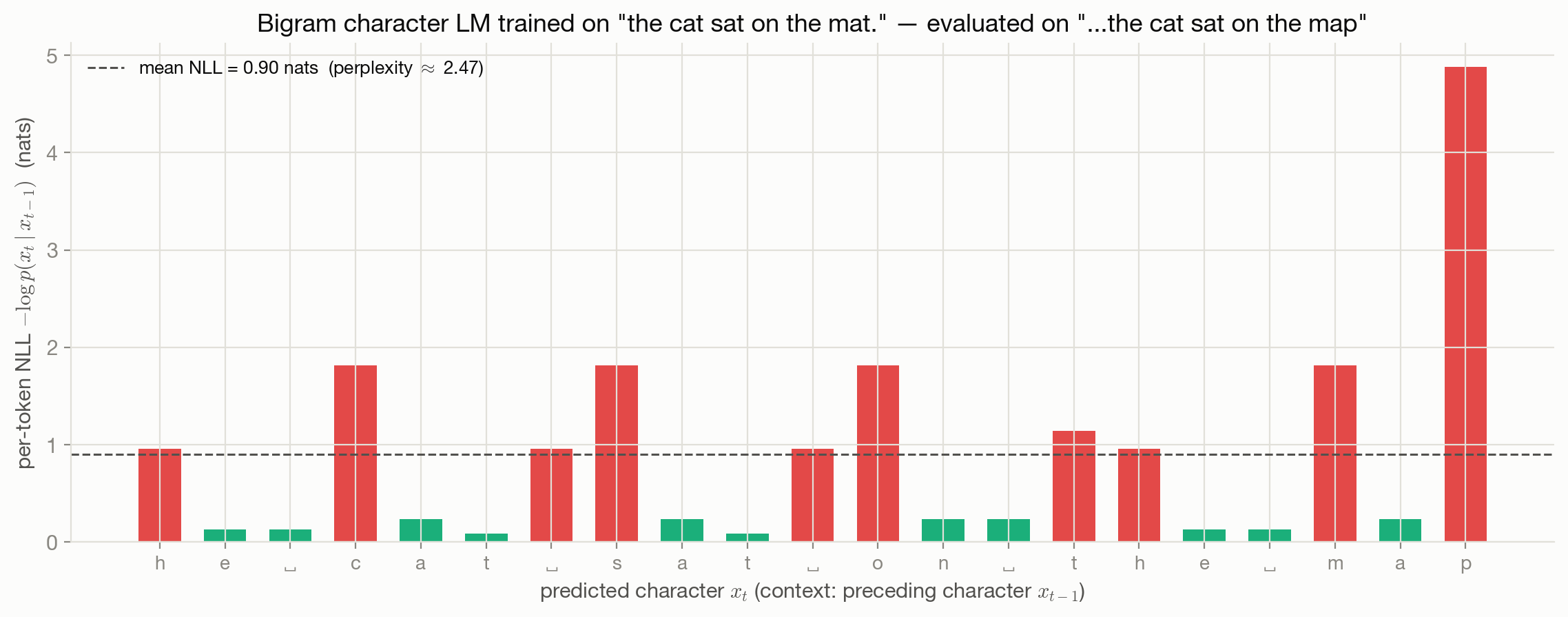
Figure 15.1 makes both the per-token sum and perplexity concrete with an actual, tiny computed example: a character-level bigram model fit by counting transitions in a short, repetitive training corpus, then evaluated token-by-token on a test sequence that mostly follows the training pattern but ends with a deliberate deviation.
15.6 Behavior and edge cases
Because each position is an ordinary softmax cross-entropy, the same asymmetry from Chapter 2 and Chapter 6 applies per-token: a confidently wrong prediction at one position is punished far more severely than a mildly-uncertain one, and this is exactly what Figure 15.1 shows as the spike at the surprising final token. A subtler edge case is specific to sequences: errors made under the model’s own generated prefix at inference time can compound, since a bad token at position \(t\) becomes part of the (now wrong) context for every subsequent position — a consequence of exposure bias, not something visible in the teacher-forced training loss itself, since training never actually conditions on the model’s own mistakes. Long-range dependencies are also bounded by whatever context window the parameterization uses; information further back than that window is architecturally unavailable to \(p_\theta(x_t\mid x_{<t})\), regardless of how well the objective is optimized.
15.7 Limitations
The chain-rule factorization is exact, but the overall objective is only as good as (a) the parametric family used for \(p_\theta(x_t\mid x_{<t})\) and (b) teacher forcing’s implicit assumption that training the model to predict well given true prefixes transfers to predicting well given its own, possibly imperfect prefixes at inference time. Neither gap is addressed by the NLL derivation itself; they are the reason later alignment- and RL-adjacent techniques exist on top of pure NLL pretraining (see Chapter 16). A separate, well-known limitation is that low NLL on held-out text is not the same as producing text a human judge would call good, helpful, or truthful — the likelihood objective is faithful to “predict the next token accurately,” which is a narrower target than “communicate well.”
15.8 Optimization implications
The per-position sum structure is what makes teacher-forced training practical: each sequence yields \(T\) parallelizable classification terms computed from a single forward pass, rather than \(T\) sequential steps, and the sum’s gradient is additive over positions exactly as Chapter 2’s NLL sum was additive over examples — enabling standard minibatch training with sequences (or chunks of sequences) as the unit of batching. The softmax saturation behavior flagged in Chapter 6 applies per-position here too; see Chapter 17 for gradient-conditioning comparisons across losses in this book.
15.9 Connections
- Chapter 2 supplies the exact NLL machinery this chapter reapplies to sequences — the only new content here is the chain-rule factorization and the parameterization choice, not a new derivation principle.
- Chapter 6 supplies the categorical cross-entropy this chapter uses, unchanged in form, once per position.
- Chapter 12’s Plackett–Luce construction is, structurally, the same idea as this chapter’s autoregressive factorization — a chain of categorical choices, each conditioned on what came before — applied to rankings instead of token sequences. Worth reading the two derivations side by side.
- Chapter 16 builds directly on top of this chapter: the pretrained (or instruction-tuned) model trained on this autoregressive NLL objective is the \(\pi_{\mathrm{ref}}\) — and usually the initialization for \(\pi_\theta\) — in the preference-tuning objectives derived there.