16 Preference and Alignment Objectives: From Bradley–Terry to DPO
A model pretrained on the autoregressive NLL objective of Chapter 15 produces text that is, in a precise sense, likely continuation of its training distribution — but “likely” and “what a person actually wants” are not the same target. Two continuations can both be plausible next-token sequences while one is clearly the response a person would prefer: more helpful, better formatted, less evasive. That preference is comparative by nature — a person can usually say this response is better than that one far more reliably than they can assign either response an absolute numerical quality score. This chapter works out, in real derivation detail, how a training signal built entirely from comparisons like that can be turned into a loss a language model can actually be trained on — first via the two-stage route that made this practical at scale (reward modeling plus reinforcement learning), and then via Direct Preference Optimization, which collapses that two-stage machinery into a single, direct loss with — remarkably — the exact same algebraic shape already derived twice earlier in this book.
16.1 The problem
After pretraining, choose \(\theta\) so that \(\pi_\theta\), the model’s distribution over completions \(y\) given a prompt \(x\), is more likely to produce outputs that humans prefer. The available supervision is a dataset of preference pairs: for a prompt \(x\), a preferred completion \(y^+\) and a dispreferred completion \(y^-\), written \(y^+ \succ y^-\). This target is comparative, not a scalar label or a next-token identity — none of the NLL machinery from Chapters 2, 6, or 15 applies to it directly, since none of those chapters had a notion of one whole output being preferred to another.
16.2 Assumptions
Reusing Chapter 11’s Bradley–Terry model, unchanged
The preference \(y^+ \succ y^-\) is modeled exactly the way Chapter 11 modeled \(i \succ j\) for ranked items — as a Bradley–Terry pairwise comparison (Bradley and Terry 1952) governed by some underlying scalar reward function \(r(x,y)\):
\[ P(y^+ \succ y^- \mid x) = \sigma\big(r(x,y^+) - r(x,y^-)\big). \]
This is worth stating as plainly as possible: it is the identical construction from Chapter 11, with \(y\) generalized from a ranked item to a full text completion, and the ranking score \(s_i\) replaced by a reward \(r(x,y)\). Nothing about the functional form has changed — the assumption is still that preference probability depends only on the reward gap, and grows smoothly toward certainty as that gap widens.
16.3 The RLHF lineage, briefly
The route that made preference-tuning practical at scale — reinforcement learning from human feedback (RLHF) — has two stages. This chapter covers both only briefly; the point is to establish exactly what problem DPO later collapses, not to give a full treatment of RL machinery, which stays out of scope for this book.
Stage 1: reward modeling. Fit a reward model \(r_\phi(x,y)\) by maximum likelihood under the Bradley–Terry model above, using a dataset of human preference pairs (Christiano et al. 2017; Ouyang et al. 2022):
\[ \mathcal{L}_{\mathrm{reward}}(\phi) = -\log \sigma\big(r_\phi(x,y^+) - r_\phi(x,y^-)\big). \]
It’s worth being explicit about what this step actually is: it is Chapter 11’s RankNet pairwise logistic loss, relabeled. Same Bradley–Terry likelihood, same \(-\log\sigma(\cdot)\) of a score difference, same NLL derivation — the only change is that “score of a ranked item” has become “reward of a text completion,” and the pairwise comparisons come from human preference judgments rather than from ranking supervision.
Stage 2: policy optimization. With a trained reward model in hand, optimize the language model \(\pi_\theta\) to produce completions the reward model scores highly — but not without restraint. Optimizing \(\mathbb{E}_{y \sim \pi_\theta}[r_\phi(x,y)]\) alone invites reward hacking: \(\pi_\theta\) can drift toward outputs that exploit quirks of \(r_\phi\) (which is only an imperfect proxy for real human preference) while abandoning the fluent, sensible behavior learned during pretraining. The standard fix constrains \(\pi_\theta\) to stay close, in KL divergence, to a reference policy \(\pi_{\mathrm{ref}}\) — typically the pretrained or instruction-tuned model from Chapter 15 — giving the KL-regularized objective
\[ \max_\theta\; \mathbb{E}_{y \sim \pi_\theta(\cdot\mid x)}\big[r_\phi(x,y)\big] \;-\; \beta\, D_{\mathrm{KL}}\big(\pi_\theta(\cdot\mid x)\,\|\,\pi_{\mathrm{ref}}(\cdot\mid x)\big), \]
typically optimized with an RL algorithm such as Proximal Policy Optimization (Schulman et al. 2017), since \(y\) is discrete and sampled, not something with a closed-form gradient through \(r_\phi\). This objective is the correct target — but it requires training and maintaining a separate reward model, and running genuine RL (sampling from \(\pi_\theta\), estimating a policy gradient, dealing with its variance and instability) on top of it. Both are real engineering and stability costs.
16.4 The DPO derivation
Direct Preference Optimization (Rafailov et al. 2023) asks a sharp question about the two-stage recipe above: does the KL-regularized objective’s own structure make the reward model and the RL step avoidable? The answer is yes, and the derivation is short enough to walk through in full.
Step 1: the closed-form optimal policy
For a fixed reward function \(r\), the KL-regularized objective above has a known closed-form solution. Fixing \(x\) and writing the objective as a functional of the distribution \(\pi_\theta(\cdot\mid x)\),
\[ \max_{\pi_\theta}\; \mathbb{E}_{y\sim\pi_\theta}[r(x,y)] - \beta D_{\mathrm{KL}}\big(\pi_\theta(\cdot\mid x) \,\|\, \pi_{\mathrm{ref}}(\cdot\mid x)\big), \]
is maximized by
\[ \pi^\star(y \mid x) = \frac{1}{Z(x)}\, \pi_{\mathrm{ref}}(y\mid x)\, \exp\!\left(\frac{r(x,y)}{\beta}\right), \qquad Z(x) = \sum_{y} \pi_{\mathrm{ref}}(y\mid x)\exp\!\left(\frac{r(x,y)}{\beta}\right). \]
This is a standard result from KL-regularized control / variational inference (it’s the same exponential-tilting form that shows up whenever a KL penalty toward a reference measure is combined with a linear reward term) — the optimal policy reweights the reference policy by the exponentiated, \(\beta\)-scaled reward, renormalized by \(Z(x)\). The role of \(\beta\) is visible already: a large \(\beta\) makes the exponential factor close to flat, pulling \(\pi^\star\) toward \(\pi_{\mathrm{ref}}\); a small \(\beta\) lets the reward term dominate, pulling \(\pi^\star\) toward reward-maximizing completions regardless of how far that strays from \(\pi_{\mathrm{ref}}\).
Step 2: invert it to express the implicit reward
\(Z(x)\) is generally intractable — it’s a sum (or integral) over every possible completion \(y\) — which is exactly why this closed form isn’t directly usable as a training target for \(\pi_\theta\) on its own. But the relationship between \(\pi^\star\) and \(r\) can be inverted algebraically. Solving the equation above for \(r(x,y)\):
\[ r(x,y) = \beta \log\frac{\pi^\star(y\mid x)}{\pi_{\mathrm{ref}}(y\mid x)} + \beta \log Z(x). \]
Relabel \(c(x) := \beta\log Z(x)\) — a term that depends on \(x\) alone, not on \(y\) — and read this equation the other way around: any policy \(\pi_\theta\) implicitly defines a reward function via
\[ r(x,y) = \beta \log\frac{\pi_\theta(y\mid x)}{\pi_{\mathrm{ref}}(y\mid x)} + c(x). \]
This is the crux of the whole derivation. It says the reward isn’t a separate object that has to be learned by a separate network — it’s recoverable, up to the unknown, \(y\)-independent constant \(c(x)\), directly from the log-probability ratio between the trained policy and the reference policy.
Step 3: substitute into Bradley–Terry — the constant cancels
Plug this implicit reward into the Bradley–Terry preference model from the top of this chapter. The model only ever needs a difference of rewards, \(r(x,y^+) - r(x,y^-)\), and \(c(x)\) is the same for both terms of that difference (it depends on \(x\), not on \(y^+\) or \(y^-\)) — so it cancels exactly:
\[ r(x,y^+) - r(x,y^-) = \beta\log\frac{\pi_\theta(y^+\mid x)}{\pi_{\mathrm{ref}}(y^+\mid x)} - \beta\log\frac{\pi_\theta(y^-\mid x)}{\pi_{\mathrm{ref}}(y^-\mid x)}. \]
\(Z(x)\) — the intractable sum over all completions — never has to be computed. Substituting this difference into \(P(y^+\succ y^- \mid x) = \sigma(r(x,y^+) - r(x,y^-))\) and taking the negative log-likelihood exactly as in Chapter 11’s RankNet derivation produces a loss expressed entirely in terms of \(\pi_\theta\) and \(\pi_{\mathrm{ref}}\) — no reward model, no sampling from \(\pi_\theta\), no RL step:
\[ \mathcal{L}_{\mathrm{DPO}}(\theta) = -\log\sigma\!\left(\beta\log\frac{\pi_\theta(y^+\mid x)}{\pi_{\mathrm{ref}}(y^+\mid x)} - \beta\log\frac{\pi_\theta(y^-\mid x)}{\pi_{\mathrm{ref}}(y^-\mid x)}\right). \]
The closing move
Look at what this is. It is, once again, exactly Chapter 11’s pairwise logistic loss \(-\log\sigma(\Delta)\) — the same Bradley–Terry NLL that appeared as RankNet in Chapter 11 and as the reward-model loss earlier in this very chapter — with the “score difference” \(\Delta\) now built not from a learned scalar score \(s_i - s_j\), nor from a separately trained reward \(r_\phi(x,y^+) - r_\phi(x,y^-)\), but from a difference of log-probability ratios between the policy being trained and a fixed reference policy. DPO’s insight is not a new loss function — it’s the observation that the reward in the Bradley–Terry model was always implicit in some policy (via the closed-form relationship of Step 1), so a policy can be trained directly against preference data by treating its own log-probability ratio to \(\pi_{\mathrm{ref}}\) as that implicit reward, skipping the reward-model training and the RL policy-optimization step entirely.
16.5 The resulting objective
\[ \mathcal{L}_{\mathrm{DPO}}(\theta) = -\log\sigma\!\left(\beta\log\frac{\pi_\theta(y^+\mid x)}{\pi_{\mathrm{ref}}(y^+\mid x)} - \beta\log\frac{\pi_\theta(y^-\mid x)}{\pi_{\mathrm{ref}}(y^-\mid x)}\right) \]
This is a genuine, textbook example of what “hybrid” means in this book’s taxonomy — not a vague middle ground, but a loss with two distinct, traceable origins that were combined by an exact derivation. It is decision-theoretic: it starts from a KL-regularized expected-reward objective, the same reward-maximization-under-a-penalty structure that governs RL and control problems. It is also derived from likelihood: the Bradley–Terry model it is substituted into, and the NLL taken of it, is the same likelihood-based construction as Chapter 11’s RankNet. Neither half is a decoration on the other — the KL-regularized objective is what produces the closed-form \(\pi^\star\) that makes the reward implicit, and the Bradley–Terry NLL is what turns that implicit reward into a trainable loss.
16.6 What \(\beta\) and the KL term actually do
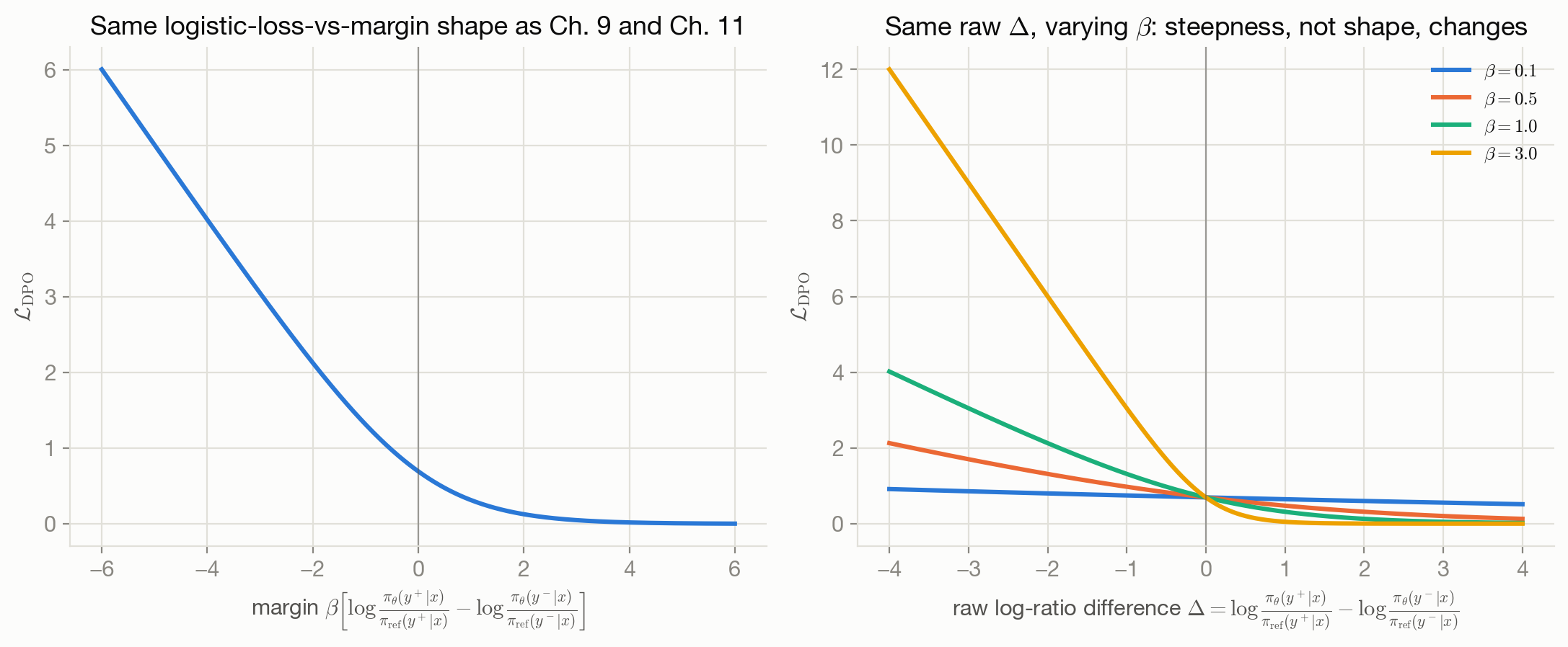
\(\beta\) is not merely a learning-rate-like scale factor on the loss — it sets the trade-off between satisfying the observed preferences and staying close to \(\pi_{\mathrm{ref}}\), visible directly in the closed-form \(\pi^\star \propto \pi_{\mathrm{ref}}\exp(r/\beta)\) from Step 1: small \(\beta\) lets the reward term dominate, permitting \(\pi_\theta\) to move far from \(\pi_{\mathrm{ref}}\) in pursuit of the preference signal; large \(\beta\) keeps \(\pi_\theta\) close to \(\pi_{\mathrm{ref}}\) regardless of what the preference data says. This is the same regularization-strength theme Chapter 3 introduced for the prior’s variance/scale parameter — there, the prior pulled a point estimate toward zero or toward a mode, with strength set by \(\tau^2\) or \(b\); here, \(\pi_{\mathrm{ref}}\) plays the role of the “prior” a policy is regularized toward, and \(\beta\) plays the role Chapter 3’s \(\lambda\) played, with the same qualitative behavior: too little regularization risks overfitting to (or exploiting quirks of) the training signal, too much makes the training signal nearly irrelevant.
Figure 16.1 plots the DPO loss against this \(\beta\)-scaled margin directly, and shows both that its shape is the by-now-familiar logistic curve and how \(\beta\) rescales a fixed amount of raw preference signal into a steeper or shallower effective push.
16.7 Interpretation
Minimizing \(\mathcal{L}_{\mathrm{DPO}}\) pushes \(\beta\log\frac{\pi_\theta(y^+\mid x)}{\pi_{\mathrm{ref}}(y^+\mid x)}\) above \(\beta\log\frac{\pi_\theta(y^-\mid x)}{\pi_{\mathrm{ref}}(y^-\mid x)}\) — that is, it increases the preferred completion’s probability relative to the reference model’s probability for it, and decreases the dispreferred completion’s probability relative to the reference model’s probability for it. It does not directly require \(\pi_\theta(y^+\mid x) > \pi_\theta(y^-\mid x)\) in absolute terms; what matters is the ratio to \(\pi_{\mathrm{ref}}\), which is precisely what keeps the objective tied to the reference model’s own sense of plausible continuations rather than rewarding \(y^+\) merely for having high raw probability under some degenerate policy.
16.8 Behavior and edge cases
As with RankNet, a pair that is already correctly and confidently ordered (large positive margin) contributes a vanishing gradient, while a mis-ordered or barely-separated pair pulls hard — the same saturating \(\sigma(-\Delta)\)-shaped pull derived in Chapter 11, now acting on log-probability ratios. Because the loss only ever depends on a difference of log-ratios, adding any constant shift to both \(\log\pi_\theta(y^+\mid x)\) and \(\log\pi_\theta(y^-\mid x)\) leaves the loss unchanged — mirroring RankNet’s invariance to a constant shift in all of an item’s scores. A practically important edge case: if \(\pi_\theta\) drifts far enough from \(\pi_{\mathrm{ref}}\) that the log-ratios become very large in magnitude, gradients can behave erratically; this is part of why DPO training in practice still benefits from a well-chosen \(\beta\) and a reasonable initialization at \(\pi_\theta = \pi_{\mathrm{ref}}\).
16.9 Limitations
DPO inherits Chapter 11’s Bradley–Terry assumption wholesale: preference probability is assumed to depend only on the reward gap, which can be violated by inconsistent or non-transitive human preferences. It also inherits a subtler issue from the derivation itself: the closed-form \(\pi^\star\) in Step 1 is exact only for the true reward function and exact KL-regularized optimization; DPO substitutes the model’s own implicit reward and optimizes it directly by gradient descent on a finite preference dataset, which is a different (and in practice, generally more stable, but not provably identical) procedure from running the two-stage RLHF pipeline to convergence. And, as with the reward model it replaces, DPO is only as good as the preference data it’s trained on — it has no separate mechanism for detecting when human raters themselves disagree, are inconsistent, or are rewarding a superficial trait (e.g. verbosity) rather than the intended quality.
16.10 Optimization implications
DPO’s loss is Chapter 11’s smooth, convex-in-the-margin logistic loss, applied to a quantity — the log-ratio difference — that is straightforward to compute from two forward passes (one for \(\pi_\theta\), one, often precomputed and frozen, for \(\pi_{\mathrm{ref}}\)) per preference pair, with ordinary backpropagation. This is precisely what makes it dramatically simpler to implement than the RLHF pipeline it replaces: no policy-gradient variance, no separate reward-model training loop, no RL-specific stability tricks. See Chapter 17 for how this compares more generally to the other losses in this book in terms of gradient behavior.
16.11 Connections
- Chapter 11 supplies the Bradley–Terry model and the pairwise logistic loss this chapter reuses essentially verbatim — twice, once for the reward model and once, after the substitution, for DPO itself.
- Chapter 15 supplies \(\pi_{\mathrm{ref}}\), typically the pretrained or instruction-tuned model from that chapter’s autoregressive NLL objective, and often the initialization for \(\pi_\theta\) as well.
- Chapter 3 established the regularization-strength theme echoed here by \(\beta\): a penalty that pulls an estimate toward a reference (there, a prior over \(\theta\); here, \(\pi_{\mathrm{ref}}\)), with strength as an explicit, tunable trade-off.
- Chapter 9 is a third, independent route to the same logistic-loss family — worth comparing all three derivations (surrogate/margin, Bradley–Terry ranking, and this chapter’s KL-regularized-reward substitution) side by side as an illustration of how differently-motivated reasoning can converge on the identical formula.
- Chapter 18 can use this chapter as a current, non-trivial capstone case study: DPO is a real, widely deployed objective that emerged from composing a decision-theoretic (KL-regularized reward maximization) argument with a likelihood-based (Bradley–Terry NLL) one, exactly the kind of synthesis that chapter’s design recipe asks a reader to attempt for a new problem.