11 Pairwise Ranking: RankNet
The most direct way to use ranking supervision is to stop trying to predict an absolute relevance value for each item and instead ask a narrower question the data usually answers more reliably anyway: for a pair of items, which one should rank higher? Search logs, comparison judgments, and click data all naturally produce statements of the form “item \(i\) should outrank item \(j\)” — pairwise preferences — even when no one ever assigned either item a clean absolute relevance score. RankNet turns exactly this kind of supervision into a training objective, and it does so by a route that should look familiar: write down a probabilistic model of the preference, then take its negative log-likelihood.
11.1 The problem
Given a set of observed pairwise preferences \(i \succ j\) over items scored by \(s_i = f_\theta(x_i)\), choose \(\theta\) so that the induced scores respect as many of the observed preferences as possible — ideally with a wide, confident separation between preferred and dispreferred items rather than a narrow one.
11.2 Assumptions
Model each preference probabilistically rather than treating it as a hard constraint: assume the probability that \(i\) is preferred to \(j\) is a function of the difference between their scores,
\[ P(i \succ j) = \sigma(s_i - s_j), \qquad \sigma(z) = \frac{1}{1+e^{-z}}. \]
This is worth naming precisely: it is the Bradley–Terry model for paired comparisons (Bradley and Terry 1952), originally developed for ranking competitors from win/loss records, written here in log-score form with \(s_i - s_j\) playing the role of a log-odds. The same construction reappears, essentially unchanged, in Chapter 16’s treatment of language-model preference data — worth remembering this name now.
The assumption is doing real work: it says preference probability depends only on the score gap, is symmetric in a specific way (\(P(i\succ j) = 1-P(j\succ i)\), since \(\sigma(-z)=1-\sigma(z)\)), and grows toward certainty smoothly as the gap widens rather than jumping discontinuously. It does not assume preferences are transitive across items, and in practice they need not be perfectly consistent in the data — the model just says how to score whatever pairs are observed.
11.3 Derivation
For an observed preference \(i \succ j\) — encode it as target \(1\) under this Bernoulli model — the likelihood of that single observation is \(P(i\succ j) = \sigma(s_i - s_j)\), and its negative log-likelihood is, by exactly the same Bernoulli-NLL algebra as Chapter 6:
\[ -\log \sigma(s_i - s_j) = \log\big(1 + e^{-(s_i-s_j)}\big). \]
This is not a new formula. It is Chapter 9’s logistic loss, with the margin filled in as a score difference \(s_i-s_j\) rather than a single classification margin \(y\cdot z\) — the same sigmoid/log-odds construction from Chapter 6, applied one level up to a comparison between two items instead of a single label.
The original RankNet paper (Burges et al. 2005) states a slightly more general form, useful when preferences come with uncertainty (near-ties, or annotator disagreement) rather than as hard 0/1 judgments: let \(\bar P_{ij} \in [0,1]\) be the target probability that \(i \succ j\) (typically \(1\), \(0.5\) for a stated tie, or something empirical), and use ordinary cross-entropy against it,
\[ \ell_{ij} = -\bar P_{ij}\log P_{ij} - (1-\bar P_{ij})\log(1-P_{ij}), \qquad P_{ij} = \sigma(s_i-s_j). \]
Setting \(\bar P_{ij}=1\) recovers the formula above exactly.
11.4 The resulting objective
For a set of observed preference pairs \(\mathcal{P}\) (each with target \(\bar P_{ij}\), usually \(1\)): \[ \ell_{\mathrm{RankNet}}(\theta) = \sum_{(i,j)\in\mathcal{P}} \Big[-\bar P_{ij}\log\sigma(s_i-s_j) - (1-\bar P_{ij})\log\big(1-\sigma(s_i-s_j)\big)\Big] \]
RankNet’s loss is the negative log-likelihood of a Bradley–Terry pairwise preference model — not a distance-based or margin-based heuristic invented for ranking specifically. The apparent novelty is entirely in what’s being modeled (a preference between two items) rather than in the loss formula itself, which is Chapter 6’s Bernoulli NLL one more time.
11.5 Interpretation
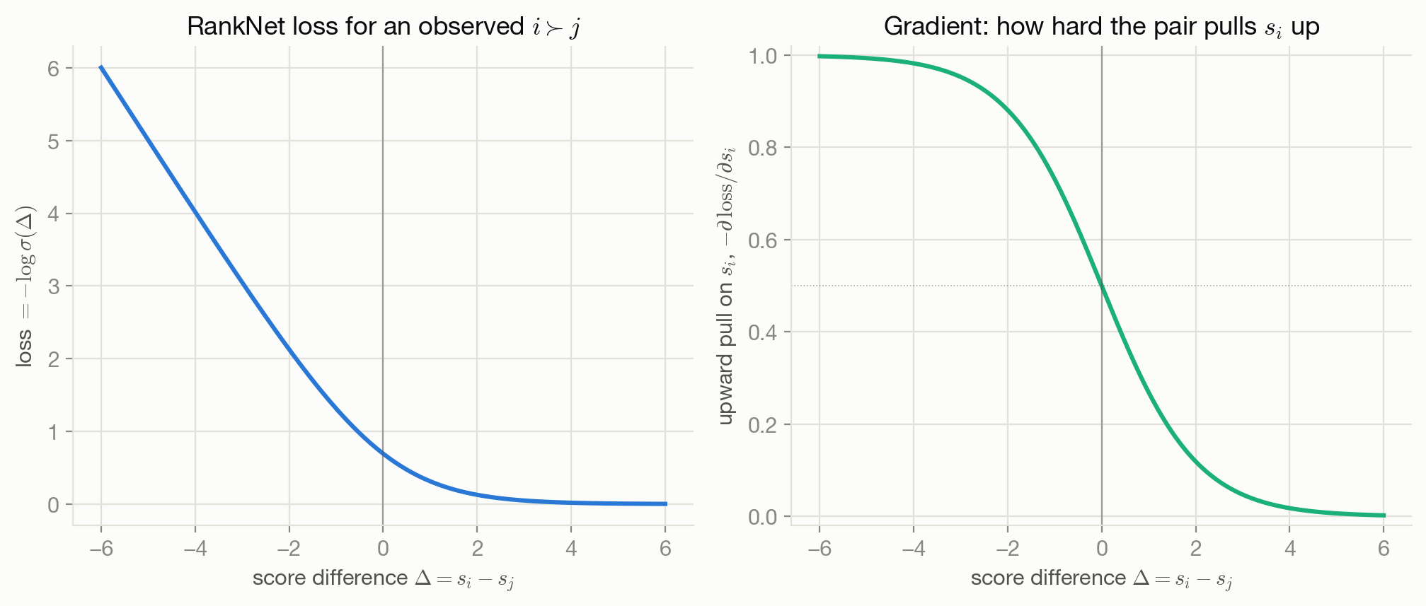
Minimizing \(\ell_{\mathrm{RankNet}}\) pushes \(s_i - s_j\) positive and large whenever \(i \succ j\) is observed — not merely positive. Because the loss is \(\log(1+e^{-\Delta})\) rather than a hard threshold, a pair that’s already correctly and confidently separated contributes almost nothing further to the gradient, while a pair that’s wrongly ordered or barely separated contributes a strong pull. The score \(s_i\) itself has no absolute meaning here — only differences between scores matter, since the loss is invariant to adding the same constant to every item’s score.
11.6 Behavior and edge cases
Figure 11.1 shows the loss and its pull on \(s_i\) as functions of the score difference \(\Delta = s_i - s_j\). The pull — the magnitude of \(-\partial\,\text{loss}/\partial s_i\) — is exactly \(\sigma(-\Delta)\): close to \(1\) (a strong upward push on \(s_i\)) when the pair is currently mis-ranked (\(\Delta \ll 0\)), and close to \(0\) (almost no push) once the pair is already well-separated in the correct order (\(\Delta \gg 0\)). This is the same saturating-gradient behavior Chapter 6 flagged for cross-entropy generally: confidently-wrong pairs get corrected hardest; already-correct pairs are left alone.
11.7 Limitations
RankNet only ever compares items within an observed pair — it has no mechanism to know that correctly ordering the top two search results matters more than correctly ordering results 40 and 41; every violated pair contributes to the loss on equal footing regardless of where in the final ranking it ends up. Chapter 13 exists specifically to patch this gap. Pair construction from graded relevance judgments is also a real design decision (which pairs to sample, how many per query) that this chapter’s formula is silent about, and a poor sampling strategy can bias what the model learns even though the pairwise loss itself is well-specified.
11.8 Optimization implications
The loss is convex in \(\Delta\) (it’s Chapter 9’s logistic loss) and smooth everywhere, so pairwise RankNet training behaves like ordinary logistic regression on constructed pair-difference features — no new optimization difficulty is introduced by moving from single-example classification to pairwise ranking. See Chapter 17 for the general comparison of loss curvature and conditioning.
11.9 Connections
- Chapter 9 supplies the exact loss formula this chapter reuses on a score difference instead of a single margin.
- Chapter 6 supplies the sigmoid/log-odds derivation pattern this chapter applies one level up.
- Chapter 16 reuses the Bradley–Terry model named here essentially unchanged, comparing full text completions instead of ranked items.
- Chapter 12 is the listwise alternative to this pairwise decomposition.
- Chapter 13 directly extends this chapter’s gradient with metric-aware weighting (LambdaRank).