1 The Learning Problem
Every supervised learning method, from linear regression to a trillion- parameter language model, is doing the same abstract thing: producing a function that maps inputs to predictions, and being told, somehow, whether those predictions are good. The “somehow” is the subject of this entire book. Before asking where cross-entropy or squared error come from, it’s worth being precise about the object they are instances of — because the central claim of this book is that a loss function is not an arbitrary formula bolted onto a model. It is part of how the learning problem itself is defined.
1.1 The pieces of a learning problem
A supervised learning problem starts with an input \(x \in \mathcal{X}\) — a vector of pixels, a sentence, a row of a spreadsheet — and a target \(y \in \mathcal{Y}\) that \(x\) is somehow associated with: a class label, a real number, a ranked list, the next token in a sequence. The pair \((x, y)\) is assumed to be a sample from some true, unknown joint distribution \(P\) over \(\mathcal{X} \times \mathcal{Y}\). Nobody has access to \(P\) directly; what’s available is a finite dataset \(D = \{(x_i, y_i)\}_{i=1}^n\), drawn i.i.d. from it.
A model is a family of functions \(f_\theta : \mathcal{X} \to \mathcal{Z}\), indexed by parameters \(\theta\) — a weight vector, a tree structure, the entries of a neural network. \(f_\theta\) produces a raw output \(z = f_\theta(x)\): sometimes this is used directly as a point prediction \(\hat y\), sometimes it’s a logit later passed through a sigmoid or softmax, sometimes it parameterizes a full distribution. Learning means choosing \(\theta\) — using only \(D\), never \(P\) — so that \(f_\theta\) behaves well on inputs it hasn’t seen. “Behaves well” is exactly what still needs to be defined, and defining it is the job of a loss.
1.2 Error and loss
Given a prediction and a true target, an error is some raw discrepancy between them — a residual \(y - \hat y\), a mismatch between a predicted class and the true one, a disagreement between a predicted and true ranking. A loss \(\ell(\theta; x, y)\) is a number that says how much that particular error should count against \(\theta\). It is tempting to treat “error” and “loss” as synonyms, but they are not: the error is a fact about a single prediction, while the loss is a rule for turning that fact into a scalar penalty, and the same error can be turned into very different penalties depending on which rule is chosen.
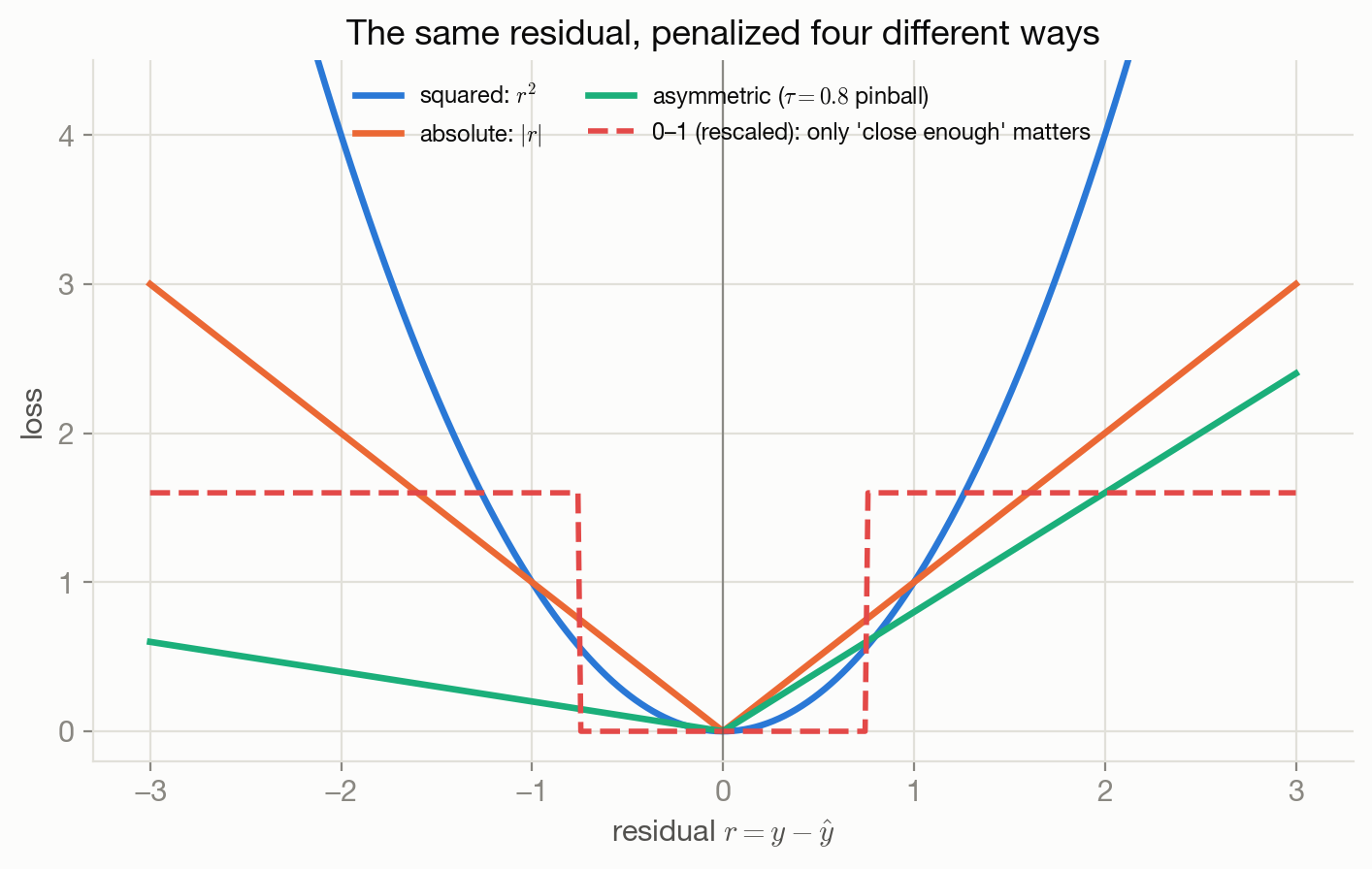
Figure 1.1 makes this concrete with four rules applied to the same residual \(r = y - \hat y\): squaring it, taking its absolute value, weighting over- and under-predictions asymmetrically, or only caring whether \(|r|\) exceeds some tolerance. At \(r = -2\), these disagree about the penalty by more than a factor of two, and the 0–1 rule doesn’t even scale with how wrong the prediction is once past the tolerance. None of the four rules is “the” objectively correct way to score that residual. Choosing between them is choosing what kind of mistake a model gets punished for making, and later chapters (4, 5, and 9 in particular) derive exactly when each choice is justified and why.
1.3 Expected risk
If a loss \(\ell\) has been chosen, the quantity that actually matters is how well \(\theta\) performs on average, over the true data distribution — including inputs that were never observed. That average is the expected risk (or population risk):
\[ R(\theta) = \mathbb{E}_{(X,Y)\sim P}\big[\ell(\theta; X, Y)\big]. \]
\(R(\theta)\) is what you would minimize if you had unlimited data and unlimited computation: it’s a property of \(\theta\) and the true world \(P\), not of any particular sample. It is also, in general, impossible to compute exactly, because \(P\) is unknown. This is the central obstacle of learning from data, and it’s worth pausing on: the thing you actually want to minimize is not the thing you can write down.
1.4 Empirical risk
What can be computed is an average over the data actually observed. The empirical risk replaces the expectation over \(P\) with an average over the \(n\) samples in \(D\):
\[ \hat R(\theta) = \frac{1}{n}\sum_{i=1}^n \ell(\theta; x_i, y_i). \]
\(\hat R(\theta)\) is a Monte Carlo estimate of \(R(\theta)\): for any fixed \(\theta\), the law of large numbers guarantees \(\hat R(\theta) \to R(\theta)\) as \(n \to \infty\), and concentration inequalities (Hoeffding’s, for bounded losses) say how fast, with high probability, for a fixed \(\theta\) evaluated on a fresh sample. This is the entire justification for the strategy nearly every ML algorithm follows, called empirical risk minimization (ERM): pick \(\hat\theta = \arg\min_\theta \hat R(\theta)\), and hope that because \(\hat R\) tracks \(R\), the minimizer of one is a good minimizer of the other.
That hope needs a caveat that the paragraph above’s LLN argument doesn’t actually cover: the guarantee is for a fixed \(\theta\) evaluated on data it didn’t choose, but ERM chooses \(\hat\theta\) by looking at \(D\), so \(\hat R(\hat\theta)\) is no longer an unbiased estimate of \(R(\hat\theta)\) — this is exactly the gap that overfitting lives in, and it’s why held-out validation data, regularization (Chapter 3), and generalization theory exist. This book does not develop that theory in depth — optimization-lab and standard statistical learning theory references cover it — but it’s worth knowing precisely which step of the argument it patches.
1.5 The loss is part of the problem, not an implementation detail
It’s common to talk about a loss function the way you’d talk about a solver setting: a knob to pick so that training converges nicely. That framing is backwards. The loss is the definition of what “a good prediction” means for this problem. Change the loss and, in general, you change what the optimal \(\theta\) is — not just how quickly training finds it. Squared error and absolute error are minimized by different statistics of the same distribution (Chapter 8 makes this exact: the mean versus the median). A model trained with the “wrong” loss for a problem can converge perfectly and still not be answering the question you meant to ask.
This is why the rest of this book insists on asking, for every loss it introduces, where does this actually come from — because the answer determines what minimizing it means, not just how easy it is to optimize.
1.6 What’s still missing
Nothing so far explains why squared error, or cross-entropy, or any specific \(\ell\) is the right choice for a given problem — only that some choice has to be made, and that the choice matters. The next two chapters supply the first, and most important, source of principled choices: treating the model as making a probabilistic claim about \(y\), and letting the loss fall out of that claim rather than being chosen by convention.
1.7 Connections
- Chapter 2 picks up exactly where this chapter stops: it shows that once \(f_\theta\) is interpreted as defining a conditional distribution \(p(y\mid x;\theta)\), a specific loss — negative log-likelihood — falls out of that interpretation rather than needing to be guessed.
- Chapter 8 returns to the “different losses want different predictions” point above and makes it precise: it derives exactly which statistic of \(Y\mid X=x\) each loss’s minimizer recovers.
- Chapter 17 picks up the empirical-risk- minimization machinery from an optimization angle: given \(\hat R(\theta)\), how the shape of \(\ell\) (its gradients, its curvature) determines how hard that minimization actually is.
- The Map places this chapter’s vocabulary — loss, risk, empirical risk — at the root of the whole book’s taxonomy.