8 Decision Theory and Proper Scoring Rules
Every loss chapter so far has treated a good prediction as a side effect of a good probabilistic model: assume a distribution for \(Y\), take its negative log-likelihood, minimize. That’s one route to a loss, but it quietly begs a question those chapters kept deferring — squared error’s minimizer is “the mean,” absolute error’s is “the median,” but why? Decision theory answers this directly, without going through a likelihood at all: it starts from the loss itself and asks what quantity of \(Y\) it is secretly asking you to report.
8.1 The problem
Chapter 1 opened with a figure showing four losses applied to the same residual, including a \(\tau=0.8\) asymmetric loss, and promised that what each one’s minimizer actually means would come later. That promise is due. Given a loss \(\ell(a,y)\) and a conditional distribution \(Y\mid X=x\), what value \(a\) does minimizing \(\mathbb{E}_{Y\mid X=x}[\ell(a,Y)]\) actually pick out? This is a different question from “where does this loss come from probabilistically” — it doesn’t need \(\ell\) to be an NLL of anything.
8.2 Assumptions
Nothing about \(Y\)’s distribution needs to be assumed — this machinery works for any distribution with a finite relevant moment/quantile. What’s assumed is the decision-theoretic setup itself: a space of possible decisions \(\mathcal{A}\), a loss \(\ell(a,y)\) scoring decision \(a\) against outcome \(y\), and the goal of minimizing conditional risk, \(\mathbb{E}_{Y\mid X=x}[\ell(a,Y)]\), at every \(x\) independently. This framework traces to Wald (Wald 1949) and is developed fully in Berger (Berger 1985).
8.3 Derivation
Squared loss recovers the mean
\[ \frac{d}{da}\,\mathbb{E}[(Y-a)^2] = \frac{d}{da}\,\mathbb{E}[Y^2 - 2aY + a^2] = -2\,\mathbb{E}[Y] + 2a. \]
Setting this to zero gives \(a^\star = \mathbb{E}[Y]\) — exactly, with no distributional assumption on \(Y\) at all. This proves what Chapter 4 stated without proof: minimizing expected squared error is asking for the conditional mean, full stop, regardless of whether \(Y\mid X\) is actually Gaussian.
Absolute loss recovers the median
\(\mathbb{E}|Y-a|\) isn’t differentiable at \(a=Y\), but its derivative exists almost everywhere: for \(a\) not equal to any point mass of \(Y\), \[ \frac{d}{da}\,\mathbb{E}|Y-a| = \mathbb{E}[\mathrm{sign}(a-Y)] = P(Y<a) - P(Y>a). \] Setting this to zero requires \(P(Y<a) = P(Y>a)\) — precisely the definition of a median of \(Y\). This proves Chapter 5’s claim the same way: no Laplace assumption needed, just the shape of absolute loss itself.
The pinball loss recovers a quantile
Generalize to an asymmetric loss with parameter \(\tau\in(0,1)\): \[ L_\tau(r) = r\big(\tau - \mathbb{1}\{r<0\}\big) = \begin{cases}\tau\, r & r\ge 0\\ (\tau-1)\,r & r<0\end{cases}, \qquad r = y-a. \] This is exactly the asymmetric loss from Chapter 1’s opening figure. The same derivative argument gives \(P(Y<a) = \tau\) at the optimum — \(a^\star\) is the \(\tau\)-quantile of \(Y\). Set \(\tau=\tfrac12\) and this collapses back to the median case above; the absolute-loss result is the special case of this one at \(\tau=1/2\), not a separate fact.
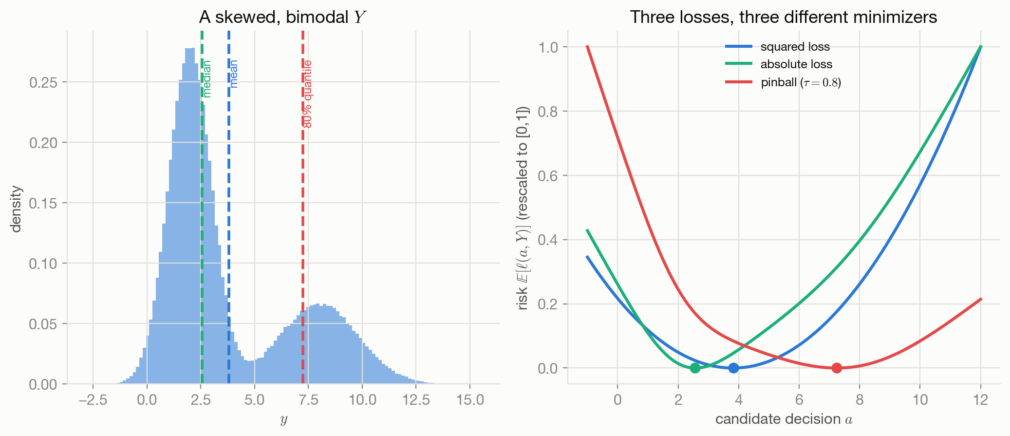
Figure 8.1 makes all three concrete on a skewed, bimodal distribution for \(Y\): the mean, median, and \(80\%\) quantile land at visibly different values (\(3.8\), \(2.6\), and \(7.2\) respectively, in the simulation shown), and each is exactly where its matching loss’s risk curve bottoms out. For a symmetric, unimodal \(Y\) these three statistics would coincide and the choice of loss would matter far less — the asymmetry here is what makes the difference visible.
Proper scoring rules
The results above concern point predictions. When the prediction itself is a full distribution \(q\) over outcomes, a scoring rule \(S(q,y)\) measures how good \(q\) was, having observed \(y\). Call \(S\) proper if reporting your true belief \(p\) is never worse in expectation than reporting any other \(q\): \[ \mathbb{E}_{Y\sim p}[S(p,Y)] \ge \mathbb{E}_{Y\sim p}[S(q,Y)] \quad \text{for all } q, \] and strictly proper if \(p\) is the unique maximizer. This is a genuinely different kind of question from anything asked so far: not “what does minimizing this loss estimate” but “does this scoring rule reward honesty, or does it reward hedging or gaming?” Gneiting and Raftery (Gneiting and Raftery 2007) is the modern reference for the theory in full.
The logarithmic score, \(S(q,y) = \log q(y)\) — i.e. negative cross-entropy — is strictly proper (its properness follows directly from Gibbs’ inequality, the same inequality behind \(D_{\mathrm{KL}}\ge 0\) in Chapter 7). The Brier score, \(S(q,y) = -\sum_k (q_k - \mathbb{1}\{y=k\})^2\), is also strictly proper (Brier 1950; Good 1952).
8.4 The resulting objective
A scoring rule \(S(q,y)\) is proper if truthfully reporting \(q=p\) maximizes \(\mathbb{E}_{Y\sim p}[S(q,Y)]\) over all \(q\), and strictly proper if \(p\) is the unique maximizer. The log score and the Brier score are both strictly proper.
The log score’s properness gives cross-entropy (Chapters 2 and 6) a second, independent justification. It was already derived as a Bernoulli or categorical negative log-likelihood — a statement about probabilistic modeling. Here it earns the same formula again from an entirely different argument: among all ways of scoring a predicted probability against an outcome, the log score is one where honesty is the uniquely optimal strategy. These are not the same fact stated twice — one is about what data the model explains, the other is about what behavior the scoring system incentivizes — and their agreement on the same formula is a real, non-obvious result, not a coincidence to skip past. The Brier score, by contrast, has no standard likelihood interpretation as a Bernoulli/ categorical NLL — its natural home is squarely here, as a proper scoring rule.
8.5 Interpretation
A proper scoring rule turns “give me your honest probability estimate” into an incentive-compatible mechanism: under a strictly proper rule, a forecaster who actually believes \(p\) has no reason to report anything else, even adversarially. This is exactly the property you want from a loss used to train a model that’s supposed to output calibrated probabilities, not just a ranking or a point guess.
8.6 Behavior and edge cases
Not every plausible-looking scoring rule is proper. A model scored (or trained) against an improper rule can have every incentive to report probabilities that are systematically over- or under-confident, because doing so scores better than honesty would — this is a real failure mode in practice, not a theoretical curiosity, and it’s why “is my loss even a proper scoring rule” is worth checking explicitly rather than assuming.
8.7 Limitations
Propriety is a property of the scoring rule in expectation over the true distribution — it says nothing about finite-sample behavior, and a proper scoring rule minimized on a small, unrepresentative dataset can still yield poorly calibrated predictions. Propriety also doesn’t imply anything about optimization difficulty: a proper scoring rule can still be non-convex or poorly conditioned in \(\theta\).
8.8 Optimization implications
Squared and absolute risk are convex in \(a\) (quadratic and piecewise-linear respectively), so their conditional minimizers are easy to locate exactly, as done numerically in Figure 8.1. Chapter 9 takes up the harder case — when the loss that matters (0–1 loss) has no usable gradient at all — and Chapter 17 returns to conditioning once more losses are on the table for direct comparison.
8.9 Connections
- Chapter 1 — this chapter is where that opening figure’s asymmetric loss gets its meaning explained.
- Chapter 4 and Chapter 5 — both left “the minimizer is the mean / the median” as an informal claim; this chapter proves it, without needing either chapter’s likelihood assumption.
- Chapters 2 and 6 — cross-entropy’s second, independent justification.
- Chapter 9 — picks up statistical consistency formally, for the harder case of classification losses that only approximate 0–1 loss.