6 Bernoulli and Categorical Likelihoods: Cross-Entropy
“Cross-entropy is defined as \(-\sum_k y_k\log p_k\)” is the sentence this book set out to avoid writing without justification. Classification asks a model to predict which of a small number of discrete outcomes occurred, and by now the pattern from Chapters 4 and 5 should be predictable: pick the probability distribution that matches the structure of \(y\), take its NLL, and see what falls out. For a two-outcome target, that distribution is Bernoulli; for a \(K\)-outcome target, categorical. Both land on formulas called “cross-entropy” — precisely because, as Chapter 7 makes exact, that name isn’t a coincidence.
6.1 The problem
\(y\) now lives in a discrete space: \(y\in\{0,1\}\) for binary classification, or \(y\in\{1,\dots,K\}\) (or one-hot in \(\mathbb{R}^K\)) for \(K\)-way classification. \(f_\theta(x)\) can’t sensibly be compared to \(y\) by subtraction the way a real-valued prediction can — what does “the prediction was off by 0.3 classes” even mean? The probabilistic reframing from Chapter 2 sidesteps the question entirely: instead of predicting a class, predict a distribution over classes, and let NLL do the rest.
6.2 Assumptions: binary case
\[ Y \sim \mathrm{Bernoulli}(p), \qquad p = \sigma(z), \quad z = f_\theta(x), \]
where \(\sigma(z) = 1/(1+e^{-z})\) is the logistic sigmoid. \(\sigma\) is not an arbitrary choice of squashing function: it is exactly the inverse of the log-odds (logit) function \(\mathrm{logit}(p) = \log\frac{p}{1-p} = z\), so the model’s raw output \(z\) is being interpreted as a log-odds — a natural, unconstrained real-valued encoding of “how much more likely class 1 is than class 0,” which \(\sigma\) then maps back into a valid probability \((0,1)\). (The choice of sigmoid specifically, versus some other monotonic map onto \((0,1)\), is closer to a design decision — motivated by exactly this clean log-odds correspondence and its resulting logistic-regression machinery — than a forced consequence of the Bernoulli assumption alone.)
6.3 Derivation: Bernoulli → binary cross-entropy
The Bernoulli probability mass function can be written in one line that covers both outcomes at once: \(p(y\mid x;\theta) = p^y(1-p)^{1-y}\) (check: at \(y=1\) this is \(p\); at \(y=0\) it’s \(1-p\)). Its negative log:
\[ -\log p(y\mid x;\theta) = -y\log p - (1-y)\log(1-p). \]
Exactly one of the two terms is active for any given \(y\): at \(y=1\), the \((1-y)\) factor zeroes out the second term and the loss is \(-\log p\); at \(y=0\), it’s \(-\log(1-p)\). This is already the familiar BCE formula, and nothing about the derivation involved a choice beyond “assume Bernoulli, take the NLL” — the same two-step recipe as every chapter so far.
6.4 Assumptions: categorical case
\[ Y \sim \mathrm{Categorical}(p_1,\dots,p_K), \qquad p_k = \mathrm{softmax}(z)_k = \frac{e^{z_k}}{\sum_{j=1}^K e^{z_j}}, \]
with \(z=f_\theta(x)\in\mathbb{R}^K\) a vector of logits, one per class. Softmax is motivated by wanting \(\log p_k\) to be linear in \(z_k\) (clean, well-behaved gradients with respect to the logits) while guaranteeing every \(p_k>0\) and \(\sum_k p_k=1\): setting \(p_k \propto e^{z_k}\) achieves both — exponentiating makes every value positive regardless of \(z_k\)’s sign, and dividing by the sum normalizes.
6.5 Derivation: categorical → cross-entropy
For a one-hot label with \(y_c=1\) at the true class \(c\) and \(0\) elsewhere, \(p(y\mid x;\theta) = \prod_k p_k^{y_k} = p_c\) — the model’s probability for whichever class actually occurred. So
\[ -\log p(y\mid x;\theta) = -\log p_c = -z_c + \log\sum_{j=1}^K e^{z_j}. \]
The middle expansion (substituting the softmax definition and using \(\log(a/b)=\log a - \log b\)) is worth doing explicitly once: it shows categorical cross-entropy reduces to “the true class’s logit, minus the log-sum-exp of every logit” — a single number computed directly from raw logits, with no need to materialize the full probability vector first.
This matters beyond elegance. Computing \(\sum_j e^{z_j}\) directly can overflow for large logits; the standard fix (the log-sum-exp trick) is to subtract \(m=\max_j z_j\) before exponentiating, \(\log\sum_j e^{z_j} = m + \log\sum_j e^{z_j - m}\), which is mathematically identical but numerically stable because every exponent is now \(\le 0\). This is exactly why deep learning frameworks fuse softmax and cross-entropy into a single numerically stable operation rather than computing \(\mathrm{softmax}\) and then \(\log\) as two separate steps — computing softmax’s normalized probabilities first and only then taking a log reintroduces the overflow/underflow risk the fused form avoids.
6.6 The resulting objectives
\[ \ell_{\mathrm{BCE}}(\theta;x,y) = -y\log\sigma(z) - (1-y)\log(1-\sigma(z)) \]
The direct Bernoulli NLL — the same construction as MSE from Gaussian and MAE from Laplace, now for a discrete target.
\[ \ell_{\mathrm{CE}}(\theta;x,y) = -z_c + \log\sum_{j=1}^K e^{z_j}, \qquad c = \text{the true class} \]
Categorical NLL under a softmax link — again a direct consequence of the distributional assumption, not a separately motivated formula that happens to resemble it.
6.7 Interpretation
Minimizing BCE or categorical cross-entropy pushes \(p_c \to 1\) for the observed class \(c\) — the model is being asked to assign as much probability mass as possible to whatever actually happened. Figure 6.1 shows the shape of that push: the loss when \(y=1\) falls smoothly toward 0 as \(p\to1\) and rises steeply as \(p\to0\), and symmetrically for \(y=0\). This is exactly Chapter 2’s general NLL asymmetry (confident-wrong is punished far harder than uncertain-wrong), specialized to two outcomes.
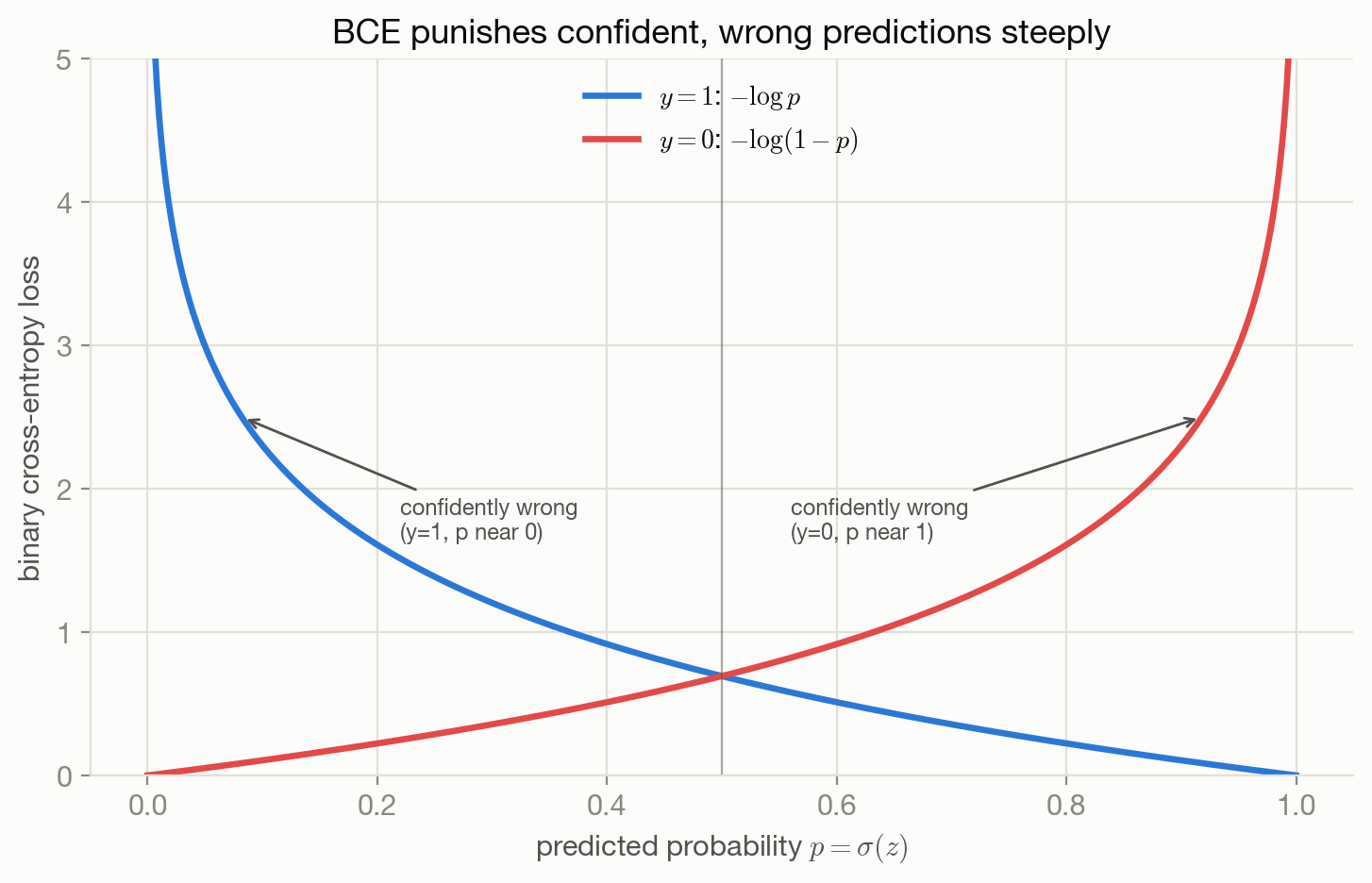
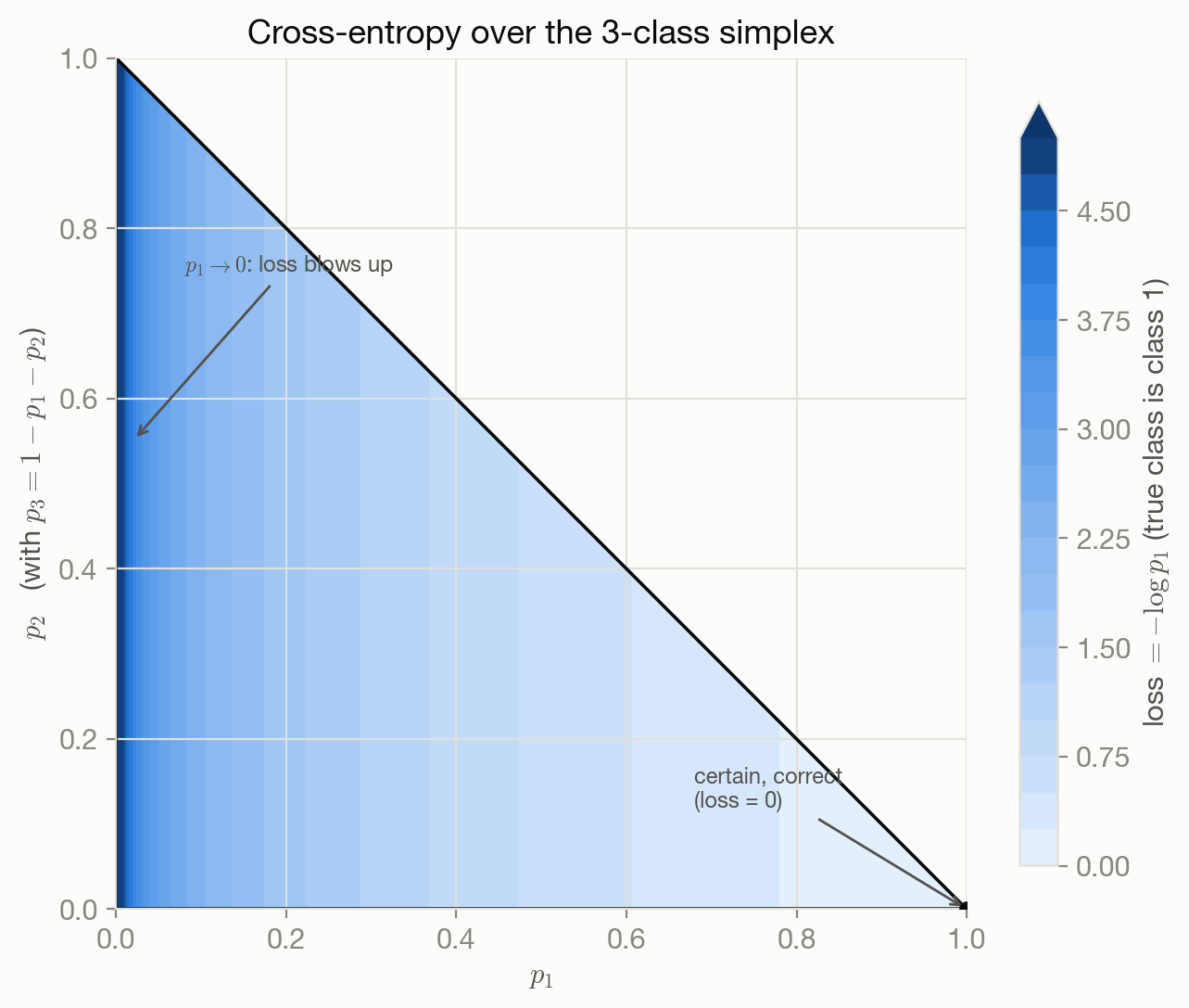
Figure 6.2 extends this to three classes, plotted directly over the probability simplex \((p_1,p_2)\) with \(p_3=1-p_1-p_2\): the loss (when the true class is class 1) is lowest at the simplex’s \(p_1=1\) corner and rises toward the opposite edge, where \(p_1\to0\).
6.8 Behavior and edge cases
Both losses are unbounded above: a model that assigns near-zero probability to the true class pays an arbitrarily large penalty, which is what drives gradient-based training away from confidently wrong predictions aggressively. At the other extreme, a model that’s correct but only mildly confident (\(p\) near 0.5–0.7) pays a small but nonzero cost — cross-entropy keeps pushing toward full certainty even after the prediction is already right, which is a real, sometimes underappreciated property (it’s part of why label smoothing exists, discussed in Chapter 7).
6.9 Limitations
Both derivations assume the label itself is noise-free and the one-hot encoding is the right target — an assumption that breaks down under label noise (some observed labels are simply wrong) or genuine class ambiguity (an example legitimately belongs partially to two classes). Neither failure makes the loss stop working mechanically, but both undermine the statistical guarantees the likelihood derivation was supposed to buy.
6.10 Optimization implications
Sigmoid and softmax both saturate: for large \(|z|\), \(\sigma'(z)\to0\) and the softmax’s gradient with respect to the dominant logit similarly flattens, so a badly-wrong, extremely confident prediction can produce a surprisingly small gradient even though the loss value itself is large — a real optimization hazard explored further in Chapter 17. This is a separate, optimization-level concern from anything derived above about the loss’s statistical meaning.
6.11 Connections
- Chapter 2 is the general machine both losses here are specific instances of.
- Chapter 7 formalizes exactly what “cross-entropy” means as an information-theoretic quantity and proves its precise relationship to KL divergence — read immediately after this one.
- Chapter 9 derives a superficially similar logistic loss from a margin/surrogate angle rather than a Bernoulli likelihood — worth contrasting the two derivations of what can look like the same formula.
- Chapter 15 reuses categorical cross-entropy token-by-token, unchanged in form, as the standard language model training objective.