3 MLE, MAP, and Regularization
Maximum likelihood asks one question: which \(\theta\) makes the observed data most probable? That question has a blind spot. It treats every candidate \(\theta\) as equally plausible before seeing any data, and with enough data that’s usually fine — but with little data, or when there’s real prior knowledge about which values of \(\theta\) are reasonable, MLE has no mechanism to use it. It will fit noise exactly as eagerly as it fits signal, because nothing in the likelihood distinguishes them. This chapter adds exactly one ingredient — a prior belief about \(\theta\) — and shows that the natural way to combine it with likelihood produces, as a direct algebraic consequence, the regularization terms already familiar from practice.
3.1 The problem
Suppose there’s a genuine prior belief about \(\theta\) before seeing any data — a physical constraint, a belief that weights are “probably small,” a previous experiment’s result. MLE has nowhere to put that belief: \(\hat\theta_{\mathrm{MLE}} = \arg\max_\theta \mathcal{L}(\theta)\) depends on \(\theta\) only through how well it explains \(D\). The question this chapter answers: what is the principled way to let a prior belief and the data jointly determine an estimate, and what does the resulting objective look like?
3.2 Assumptions
Treat \(\theta\) itself as a random variable with a prior distribution \(p(\theta)\), encoding what’s believed about it before seeing \(D\). This is the one new assumption, and it’s a substantive one: it requires being willing to express prior belief as a probability distribution, which not every problem or every practitioner is comfortable doing. Chapters 4 and 5 use \(\mathcal{N}\) and \(\mathrm{Laplace}\) distributions as likelihoods over \(y\); this chapter uses the same two distributions, but now as priors over \(\theta\) — a different role for the same mathematical objects, worth keeping straight.
3.3 Derivation
Bayes’ rule and the posterior
Given a likelihood \(p(D\mid\theta)\) and a prior \(p(\theta)\), Bayes’ rule gives the posterior — the updated belief about \(\theta\) after seeing \(D\):
\[ p(\theta \mid D) = \frac{p(D\mid\theta)\,p(\theta)}{p(D)} \;\propto\; p(D\mid\theta)\,p(\theta), \]
where \(p(D) = \int p(D\mid\theta')p(\theta')\,d\theta'\) is a normalizing constant that doesn’t depend on \(\theta\) and can be dropped for the purpose of finding the mode. Maximum a posteriori (MAP) estimation picks the single most probable value of \(\theta\) under this posterior:
\[ \hat\theta_{\mathrm{MAP}} = \arg\max_\theta p(\theta\mid D) = \arg\max_\theta \big[p(D\mid\theta)\,p(\theta)\big]. \]
Taking logs (exactly as in Chapter 2, and for the same two reasons — numerical stability and turning the product into a sum) and negating to match the minimize-a-loss convention:
\[ \hat\theta_{\mathrm{MAP}} = \arg\min_\theta \Big[\underbrace{-\log p(D\mid\theta)}_{\mathrm{NLL}(\theta)} \;-\; \log p(\theta)\Big]. \]
The first term is exactly Chapter 2’s NLL. The second is new: a penalty on \(\theta\) itself, coming entirely from the prior. Nothing about this derivation is specific to any particular prior yet — the split into “data term + prior term” is forced by the algebra of Bayes’ rule plus logarithms, for any choice of \(p(\theta)\).
Two concrete priors
Let \(\theta\) include a weight \(w\), and consider two choices.
Gaussian prior, \(w \sim \mathcal{N}(0, \tau^2)\): \(-\log p(w) = \frac{w^2}{2\tau^2} + \text{const}\) — a term proportional to \(w^2\), i.e. exactly an \(\ell_2\) penalty, matching ridge regression (Hoerl and Kennard 1970) and the classical Tikhonov regularization of ill-posed problems (Tikhonov and Arsenin 1977).
Laplace prior, \(w \sim \mathrm{Laplace}(0, b)\), with density \(\frac{1}{2b}e^{-|w|/b}\): \(-\log p(w) = \frac{|w|}{b} + \text{const}\) — a term proportional to \(|w|\), i.e. exactly an \(\ell_1\) penalty, matching the Lasso (Tibshirani 1996).
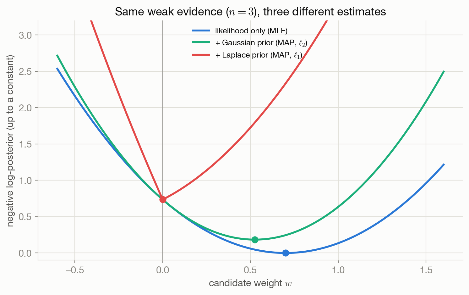
Figure 3.1 makes this concrete with \(n=3\) weakly-informative observations of a single weight (sample mean \(\bar y = 0.7\), known noise variance \(\sigma^2=1\)): the likelihood-only objective is minimized at \(\bar y\) itself; adding the Gaussian prior smoothly pulls the minimizer to \(0.525\); adding the Laplace prior instead pulls it all the way to exactly \(0\). That last number isn’t rounding — it’s the closed-form MAP estimate under a Laplace prior, \(w^\star = \mathrm{sign}(\bar y)\max(|\bar y| - \lambda, 0)\) for a threshold \(\lambda\) set by the prior’s scale \(b\) — the soft-thresholding operator behind Lasso. The Laplace density has a sharp peak at \(0\) (a kink, not a smooth maximum), and that kink is exactly what can pull a weak estimate all the way to zero rather than merely toward it; the smooth Gaussian density has no such kink and so its MAP estimate is shrunk but essentially never lands on exactly zero.
3.4 The resulting objective
\[ \hat\theta_{\mathrm{MAP}} = \arg\min_\theta \Big[\mathrm{NLL}(\theta) - \log p(\theta)\Big] \] with, for a Gaussian or Laplace prior on a weight vector \(w\), the familiar special cases \[ \arg\min_w \Big[\mathrm{NLL}(w) + \lambda \lVert w \rVert_2^2\Big] \qquad\text{or}\qquad \arg\min_w \Big[\mathrm{NLL}(w) + \lambda \lVert w \rVert_1\Big]. \]
The MAP objective itself is a direct consequence of Bayes’ rule; no part of it is a heuristic. But labeling every \(\ell_2\) or \(\ell_1\) penalty seen in practice as “secretly a prior” overclaims. The equivalence is exact only when the regularization strength \(\lambda\) is actually set to match a prior’s variance/scale (\(\lambda \propto 1/\tau^2\) or \(1/b\)) and the goal is genuinely the MAP point estimate. When \(\lambda\) is instead chosen by cross-validation to minimize held-out error — the overwhelmingly common practice — the form of the penalty still has this probabilistic reading available, but the procedure that chose \(\lambda\) is optimization-driven, not Bayesian. Call this one hybrid: a Bayesian-derived functional form, used for reasons that are often purely statistical-generalization ones.
3.5 Interpretation
\(\hat\theta_{\mathrm{MAP}}\) is the mode of the posterior — the single most probable parameter value — not its mean, and the two coincide only when the posterior is symmetric and unimodal (true for the Gaussian-prior case above, not generally true for skewed posteriors). MAP still returns one number; it discards everything else about the posterior’s shape, in particular how confident that estimate should be. A full Bayesian treatment — reporting the whole posterior \(p(\theta\mid D)\), not just its mode — is out of scope for this book, but it’s worth knowing that MAP is a waypoint on the way there, not the destination.
3.6 Behavior and edge cases
Data dominates as \(n\) grows. In the Gaussian-prior closed form \(w_{\mathrm{MAP}} = \bar y \cdot \frac{A}{A + 1/\tau^2}\) with \(A = n/\sigma^2\), the shrinkage factor \(\frac{A}{A+1/\tau^2} \to 1\) as \(n\to\infty\): the prior’s influence is diluted by data exactly the way a Beta prior’s pseudo-observations get diluted by real observations in a Beta-Binomial update. Regularization matters most precisely when data is scarce, and fades on its own as data accumulates — it is not a fixed penalty independent of how much evidence is available.
Sparsity is geometric, not accidental. The Laplace prior’s exact-zero behavior in Figure 3.1 generalizes: in higher dimensions, the \(\ell_1\) penalty’s constraint region is a polytope with corners exactly on the coordinate axes, while the \(\ell_2\) penalty’s is a smooth ball with no preferred directions — optimizing against a corner-shaped constraint tends to land exactly on a corner (some weights exactly zero), while a smooth ball almost never does. This is the same effect the 1-D closed form above shows algebraically.
3.7 Limitations
MAP inherits MLE’s blind spot for a badly misspecified likelihood, and adds a new one: a badly chosen prior can bias the estimate confidently, and unlike a well-designed likelihood (which gets corrected by more data), a sufficiently informative wrong prior can dominate for a long time. As emphasized in the origin callout above, treating every regularizer used in practice as evidence of an implicit prior is a stronger claim than the math supports — it’s a available interpretation, not a guaranteed one.
3.8 Optimization implications
Adding an \(\ell_2\) penalty keeps the objective smooth and only changes its curvature (it strictly increases it — Figure 3.1’s green curve is visibly narrower than the blue one — which is part of why ridge-regularized problems are typically better-conditioned than their unregularized counterparts). Adding an \(\ell_1\) penalty introduces a genuine non-differentiability at \(w=0\), ruling out plain gradient descent at that point and requiring subgradient methods or proximal operators (soft-thresholding is itself a proximal step) — see optimization-lab for the general machinery. Chapter 17 returns to conditioning in more depth once more losses are on the table.
3.9 Connections
- Chapter 2 is a strict special case of this chapter: MAP with a flat (improper uniform) prior is exactly MLE.
- Chapters 4 and 5 use Gaussian and Laplace distributions in the other role — as likelihoods over \(y\), producing MSE and MAE — worth contrasting directly against this chapter’s use of the same two distributions as priors over \(\theta\).
- Chapter 18 revisits “is there a prior worth encoding?” as one of the explicit questions in the recipe for designing a new objective.