9 Surrogate Losses: From 0–1 Loss to Hinge and Logistic Loss
For a binary classifier, the metric that actually matters is often embarrassingly simple: was the predicted label right or wrong. Nothing in this book’s story so far — Bernoulli likelihoods, cross-entropy, proper scoring rules — is that metric. This chapter explains why training almost never targets it directly, and what’s used instead.
9.1 The problem
Let \(y\in\{-1,+1\}\) and \(z=f_\theta(x)\) be a real-valued score, with the predicted label \(\mathrm{sign}(z)\). Define the margin \(m = y\cdot z\): positive when the prediction’s sign agrees with \(y\), negative when it doesn’t, and larger in magnitude the more confidently correct (or wrong) the prediction is. 0–1 loss is \(\ell_{0\text{-}1}(m) = \mathbb{1}\{m<0\}\) — exactly the classification error rate, averaged over examples. It is also piecewise constant: its gradient is zero everywhere it’s defined and undefined at \(m=0\), which makes gradient-based optimization of \(\hat R(\theta)\) built from it useless — a small change to \(\theta\) almost never changes any example’s sign, so almost every step has zero gradient, right up until a change is big enough to flip a sign, at which point the loss jumps discontinuously. Minimizing 0–1 loss directly is also, in the worst case, NP-hard for linear classifiers. Something else has to stand in for it during training.
9.2 Assumptions
A surrogate loss \(\varphi(m)\) is a substitute for 0–1 loss chosen so that (a) it upper-bounds 0–1 loss, \(\varphi(m) \ge \mathbb{1}\{m<0\}\), so driving \(\varphi\) down provably drives the true error rate down too, and (b) it is convex and has usable gradients almost everywhere, so ERM on \(\varphi\) is actually tractable. Nothing here assumes a likelihood or a prior — this is a different kind of justification than Parts II–IV of this book, chosen for tractability with a provable relationship to the thing that’s actually wanted.
9.3 Derivation
Hinge loss, from wanting a margin
Correctness alone (\(m>0\)) is a weak requirement — a classifier can sit arbitrarily close to the decision boundary and still be “correct.” Support vector machines (Cortes and Vapnik 1995) ask for more: a margin of at least 1, penalizing any shortfall linearly and charging nothing once the margin requirement is met: \[ \varphi_{\mathrm{hinge}}(m) = \max(0,\, 1-m). \] This is \(0\) once \(m\ge 1\), and grows linearly as \(m\) drops below \(1\) — including for already-correct-but-unconfident predictions (\(0<m<1\)), which still get penalized. It upper-bounds 0–1 loss everywhere: at \(m<0\), \(\max(0,1-m) \ge 1 = \mathbb{1}\{m<0\}\); at \(m\ge 0\), the bound is trivial since \(\ell_{0\text{-}1}=0\).
Logistic loss is binary cross-entropy, rewritten
Chapter 6 derived binary cross-entropy for \(y\in\{0,1\}\) and \(p=\sigma(z)\): \(-y\log p - (1-y)\log(1-p)\). Rewrite it in the \(\{-1,+1\}\) margin convention. Using \(\sigma(z) = 1/(1+e^{-z})\) and \(1-\sigma(z)=\sigma(-z)\), the two cases \(y=1\) and \(y=-1\) (relabeling \(y=0\to y=-1\)) both collapse into one expression: \[ -\log\sigma(yz) = \log\big(1+e^{-yz}\big) = \log\big(1+e^{-m}\big) =: \varphi_{\mathrm{logistic}}(m). \] This is not a new formula — it is Chapter 6’s binary cross-entropy, in a different but equivalent notation, now visibly a function of the margin \(m=yz\) alone rather than of \(y\) and \(p\) separately. It’s smooth: differentiable at every \(m\), including \(m=1\) where hinge has a kink.
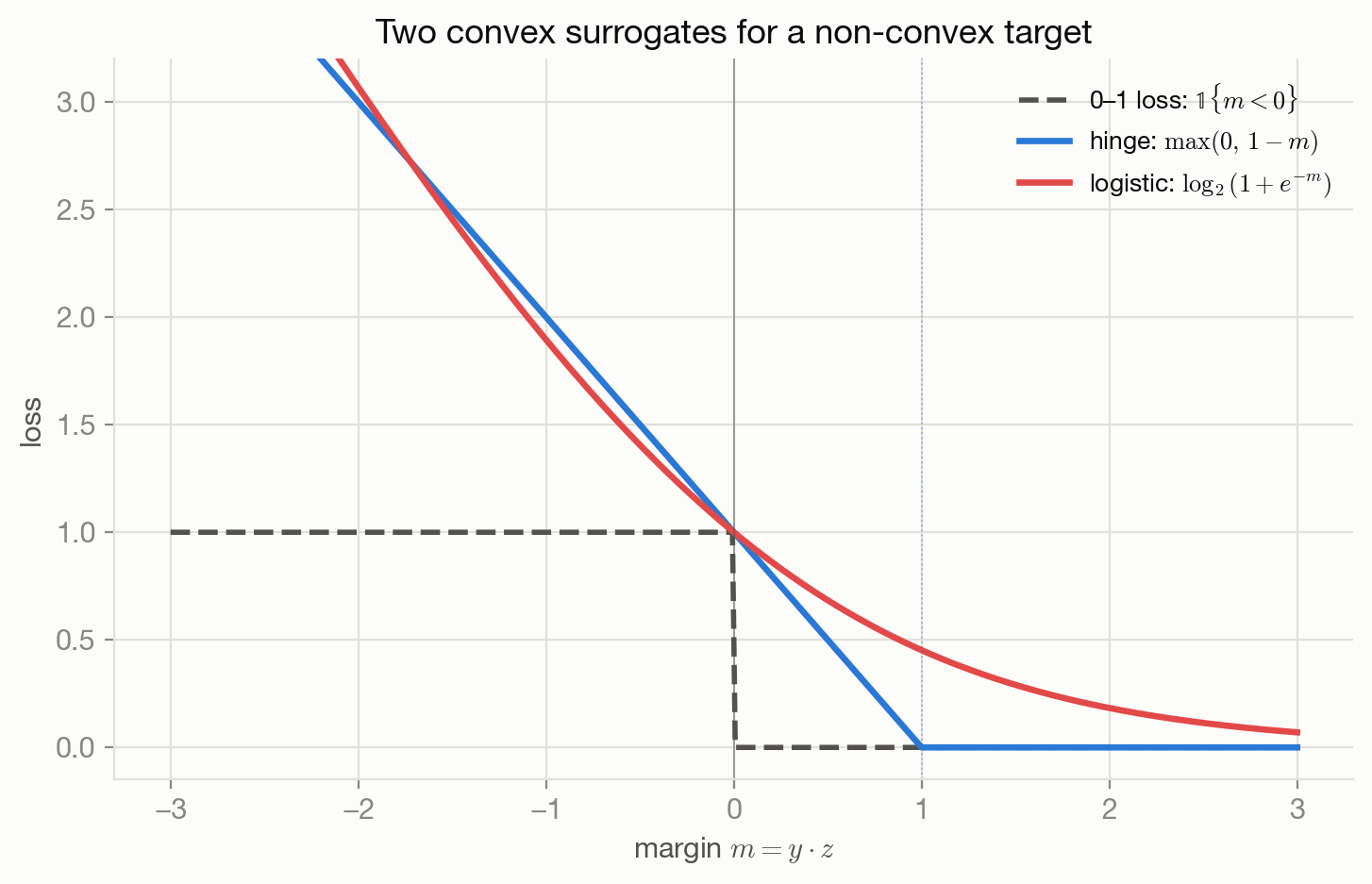
Unlike hinge, \(\log(1+e^{-m})\) does not literally upper-bound 0–1 loss with the natural log used everywhere else in this book: at, say, \(m=-0.2\), \(\log(1+e^{0.2})\approx 0.80\), strictly below \(\mathbb{1}\{m<0\}=1\). Hinge’s bound needed no such care because it has no logarithm in it to rescale. A literal, everywhere upper bound is recoverable for the logistic surrogate — switch to \(\log_2\), i.e. divide by \(\ln 2\) — and Figure 9.1 plots exactly that rescaled version for a fair visual comparison against hinge and 0–1 loss. The rescaling changes nothing that matters statistically: a positive constant multiple of a valid surrogate is still convex and still classification-calibrated (below), so both the natural-log form used in the definition box and Chapter 6, and the \(\log_2\) form plotted here, are “the same surrogate” for every purpose except a literal pointwise bound.
9.4 The resulting objective
\[ \varphi_{\mathrm{hinge}}(m) = \max(0,\,1-m), \qquad \varphi_{\mathrm{logistic}}(m) = \log(1+e^{-m}), \qquad m = y\cdot f_\theta(x). \] Both are convex. Hinge upper-bounds 0–1 loss \(\mathbb{1}\{m<0\}\) exactly as written; logistic loss upper-bounds it too, once rescaled to \(\log_2\) (a positive constant factor that changes nothing about convexity or consistency — see the derivation above).
Hinge loss has one clean justification: it’s a tractable, convex relaxation of 0–1 loss, designed for margin-maximization, with no probabilistic derivation as a likelihood of anything standard. Logistic loss is different — it has two correct derivations that happen to produce the identical formula: Chapter 6’s likelihood argument (Bernoulli NLL) and this chapter’s surrogate argument (a smooth, convex surrogate for 0–1 loss). Neither derivation is more “real” than the other; which one is relevant depends on whether you care about calibrated probabilities (the likelihood reading) or just a tractable stand-in for classification error (the surrogate reading).
9.5 Interpretation
Figure 9.1 puts 0–1 loss, hinge, and logistic loss (\(\log_2\) form, so the bound comparison below is exact — see the derivation above) on the same axes as functions of the margin. Both surrogates sit above the 0–1 step everywhere, confirming the upper-bound property visually; hinge is exactly linear beyond the kink at \(m=1\) and exactly flat (zero) beyond it, while logistic loss decays smoothly and never reaches exactly zero for finite \(m\) — a classifier trained on logistic loss keeps getting a (shrinking) gradient signal to push already-correct predictions to be even more confident, whereas one trained on hinge loss stops caring entirely once the margin requirement is met.
9.6 Behavior and edge cases
Because both surrogates are convex upper bounds, driving either one’s empirical average to a small value provably bounds the true 0–1 error rate from above — this is the entire practical justification for training on a surrogate at all. Statistical consistency makes this precise: Bartlett, Jordan, and McAuliffe (Bartlett et al. 2006) and Zhang (Zhang 2004) show that a broad class of convex margin losses, hinge and logistic among them, are classification-calibrated — under mild conditions, minimizing the surrogate’s population risk, given enough data and model capacity, recovers the Bayes-optimal 0–1 decision rule. Not every plausible surrogate has this property automatically; it has to be checked, and the papers above give the conditions.
9.7 Limitations
A surrogate’s output is not automatically a usable probability. Hinge loss’s \(z\) has no natural probabilistic scale at all — a margin of \(5\) isn’t “5 times more confident” than a margin of \(1\) in any calibrated sense. Platt scaling (Platt 1999) is the standard fix: fit a separate sigmoid on top of a trained margin classifier’s raw scores, post-hoc, to recover calibrated probabilities — a practical bridge back to Chapter 8’s proper-scoring-rule territory for a model that wasn’t trained with a calibrated probability as its objective in the first place.
9.8 Optimization implications
Hinge loss’s kink at \(m=1\) means it’s not differentiable there, requiring subgradient methods (still convex, still tractable, just not plain-gradient-friendly at that one point); logistic loss is smooth everywhere, which is part of why it’s the default in most neural classifiers even where an SVM-style margin objective would also be a valid choice. Chapter 17 compares gradient saturation between the two more directly, alongside the other losses introduced by that point.
9.9 Connections
- Chapter 6 — the exact algebraic identity between binary cross-entropy and logistic loss.
- Chapter 8 — the consistency framework this chapter specializes to the classification case, and where the probabilistic-calibration idea Platt scaling restores comes from.
- Chapter 1 — 0–1 loss reappears here from that opening figure, now as the actual target being approximated.
- Chapter 11 — RankNet’s pairwise loss is this exact logistic surrogate, applied to a difference of two scores instead of a single margin.