14 Contrastive and Metric-Learning Objectives
Every objective so far has assumed a target: a real number, a class label, an observed ranking. But a large and increasingly important slice of machine learning starts from something weaker — not “what is the right answer for this input” but “which pairs of examples are supposed to be alike, and which aren’t.” Face-recognition training data rarely comes with an absolute identity label attached to every image at training time; it comes as pairs or triplets of photos known to be the same person or different people. Self-supervised representation learning has no labels at all — only the fact that two augmented crops of the same image should end up “close” and everything else should not. This chapter asks what it means to train on relationships between examples rather than on a target for each one individually, and shows that one of the resulting objectives — InfoNCE — is not a new invention at all, but categorical cross-entropy wearing a disguise.
14.1 The problem
Given a set of examples \(x_1, \dots, x_n\) and a notion of which pairs are similar and which are dissimilar — supplied by known class identity, by data augmentation (two views of the same underlying example), or by human judgment — learn an embedding function \(f_\theta: \mathcal{X} \to \mathbb{R}^d\) so that similar pairs land close together in \(\mathbb{R}^d\) and dissimilar pairs land far apart. There is no \(y\) to predict for any single \(x_i\) in isolation; the supervisory signal is entirely relational. The object being optimized for is a geometry — a usable notion of distance or similarity in embedding space — not a point prediction or a class posterior.
14.2 Assumptions
Nothing here starts from a probabilistic model of \(y\) the way Parts II–IV did. The starting point is instead a geometric desideratum: embeddings of similar pairs should have small distance (or high similarity), embeddings of dissimilar pairs should have distance at least some margin, and — for InfoNCE specifically — a comparison between one genuine match and several non-matches can be treated as a small classification problem. This last move is the one that reconnects this chapter to the likelihood machinery of Chapter 6, and it’s worth flagging up front: it’s a genuine but nontrivial reframing, not something forced by the geometric goal alone.
14.3 Derivation
Contrastive loss: pull together, push apart
The original formulation, due to Hadsell, Chopra, and LeCun (Hadsell et al. 2006), takes a pair \((x_i, x_j)\) with a binary label \(y_{ij}=1\) if similar and \(y_{ij}=0\) if dissimilar, and a distance \(d_{ij} = \lVert f_\theta(x_i) - f_\theta(x_j)\rVert\) in embedding space. The loss charges similar pairs for being far apart, and dissimilar pairs for being closer than a margin \(\mu\):
\[ \ell_{\mathrm{contrastive}}(x_i, x_j, y_{ij}) = y_{ij}\, d_{ij}^2 + (1-y_{ij})\, \max(0,\, \mu - d_{ij})^2. \]
The first term is an ordinary squared-distance pull, unbounded — it keeps shrinking as long as similar points aren’t literally coincident. The second term is a hinge on distance, directly structurally analogous to the hinge loss of Chapter 9: it charges nothing once \(d_{ij} \ge \mu\), and a quadratic penalty for any shortfall below the margin. This design wasn’t derived from a distributional assumption about \(y_{ij}\); it was chosen because it produces the geometry that’s wanted — attraction with no floor, repulsion with a floor — and because the hinge shape gives dissimilar pairs a clean stopping point rather than being pushed to infinite separation.
Triplet loss: a relative version
Contrastive loss requires an absolute margin \(\mu\) that has to be calibrated to the scale of the embedding space. FaceNet (Schroff et al. 2015) sidesteps this by comparing three points at once — an anchor \(a\), a positive \(p\) known to match the anchor, and a negative \(n\) known not to — and asking only that the anchor be closer to the positive than to the negative, by at least a margin:
\[ \ell_{\mathrm{triplet}}(a,p,n) = \max\big(0,\; d(a,p) - d(a,n) + \mu\big). \]
This is, structurally, hinge loss one more time: define a “margin” quantity \(m = d(a,n) - d(a,p)\) — how much farther the negative is than the positive, which should be large and positive — and the triplet loss is exactly \(\max(0, \mu - m)\), Chapter 9’s hinge shape applied to a difference of distances instead of a difference of scores. The kinship isn’t coincidental: both losses exist for the same reason hinge loss exists in Chapter 9 — a tractable, margin-based stand-in for a discrete correctness condition (“is the right item closer than the wrong one”) that has no useful gradient on its own.
InfoNCE: cross-entropy over “which one is the positive”
Contrastive and triplet losses both operate on isolated pairs or triples. InfoNCE (Oord et al. 2018) changes the unit of comparison: given one genuine positive \(x^+\) for an anchor \(x\) and \(K\) negatives \(x^-_1,\dots,x^-_K\), treat the situation as a \((K{+}1)\)-way classification problem — which of the \(K+1\) candidates is the true positive? — and score each candidate by a similarity function \(\mathrm{sim}(x, x_k)\) (typically a scaled dot product of normalized embeddings). This reduction is worth writing out in full, because it is the entire content of the method, and once it’s written out, InfoNCE stops looking mysterious.
Treat the similarities \(z_k = \mathrm{sim}(x, x_k)\) for \(k \in \{+, -_1, \dots, -_K\}\) exactly as Chapter 6 treated logits: pass them through a softmax to get a probability that candidate \(k\) is the true match,
\[ p(k = {+} \mid x) = \frac{\exp(z_+)}{\exp(z_+) + \sum_{j=1}^K \exp(z_{-_j})}. \]
The label is known — index \(+\) is, by construction, the true class of this \((K{+}1)\)-way classification problem — so the negative log-likelihood is exactly Chapter 6’s categorical cross-entropy, evaluated at the true class \(+\):
\[ \ell_{\mathrm{InfoNCE}} = -\log \frac{\exp(z_+)}{\exp(z_+) + \sum_{j=1}^K \exp(z_{-_j})}. \]
There is no new algebra here beyond Chapter 6’s: it is literally \(-z_c + \log\sum_j e^{z_j}\) with \(c={+}\), the candidate similarities playing the role of logits, and the “class” being “which candidate is the real match.” Once this substitution is made explicit, InfoNCE is not a different kind of loss from cross-entropy — it is cross-entropy, with an unusual and cleverly chosen set of “classes” that changes from one training example to the next (a fresh random draw of \(K\) negatives every time). This reduction is what the origin tag below refers to as “derived from likelihood”: treat the \((K{+}1)\)-way match-identification problem as a genuine categorical target, and NLL under that categorical model is exactly InfoNCE.
The precursor to this idea is noise-contrastive estimation (NCE) (Gutmann and Hyvärinen 2010), which addressed a different but related problem — fitting an unnormalized probabilistic model without computing its intractable normalizing constant — by training a classifier to distinguish real data from samples drawn from a known noise distribution. InfoNCE inherits the “distinguish real from sampled” structure and the name, but its practical use case (representation learning via a \((K{+}1)\)-way matching task) and its usual derivation (the categorical cross-entropy reduction above) are more direct than NCE’s original binary noise/data classification, worth knowing as the historical link rather than an identical construction.
14.4 The resulting objectives
\[ \ell_{\mathrm{contrastive}}(x_i, x_j, y_{ij}) = y_{ij}\, d_{ij}^2 + (1-y_{ij})\, \max(0,\, \mu - d_{ij})^2 \]
There is no likelihood being maximized here — \(\mu\), the squared-distance pull, and the hinge-on-distance push are all chosen for the embedding geometry they produce, not derived from a probabilistic model of similarity. It shares its margin-based design logic directly with Chapter 9’s hinge loss: both are hand-designed penalties built around a “correct by at least this much, or pay a growing price” structure, not the NLL of any named distribution.
\[ \ell_{\mathrm{triplet}}(a,p,n) = \max\big(0,\; d(a,p) - d(a,n) + \mu\big) \]
Same family as contrastive loss above — a margin-based relaxation of a discrete relative-ordering requirement, structurally identical to Chapter 9’s hinge loss applied to a difference of distances instead of a difference of scores.
\[ \ell_{\mathrm{InfoNCE}} = -\log \frac{\exp(z_+)}{\exp(z_+) + \sum_{j=1}^K \exp(z_{-_j})}, \qquad z_k = \mathrm{sim}(x, x_k) \]
Exactly Chapter 6’s categorical cross-entropy, applied to a \((K{+}1)\)-way “which candidate is the true match” classification problem, with similarities standing in for logits. Nothing new is being invented in the loss formula — the novelty is entirely in how the classification problem is constructed (one positive, \(K\) sampled negatives, redrawn every example).
Separately from this reduction, InfoNCE has a second, more delicate theoretical property: van den Oord et al. (Oord et al. 2018) show that minimizing it lower-bounds the mutual information between the two halves of a positive pair, \(I(x; x^+)\), with the bound tightening as \(K\) grows. This is a real result, but it is a different and weaker claim than the exact identity above — the categorical cross-entropy reduction is exact for any \(K\), while the mutual-information reading is an asymptotic bound that depends on assumptions about the similarity function and the sampling distribution of negatives. Treat the cross-entropy reduction as the loss’s actual definition, and the mutual-information bound as a noteworthy property of it, not as a second derivation of the same formula.
14.5 Concrete applications, briefly
SimCLR (Chen et al. 2020) applies InfoNCE to self-supervised image representation learning: two random augmentations of the same image form the positive pair, every other image in the minibatch supplies negatives, and the resulting embeddings — trained with no labels at all — transfer well to downstream classification tasks. It is close to a direct implementation of the InfoNCE definition above, with the minibatch doubling as the source of negatives.
Supervised Contrastive Learning (Khosla et al. 2020) modifies InfoNCE to use actual class labels rather than augmentation identity to define positives: for an anchor of class \(c\), every other example of class \(c\) in the batch counts as a positive (not just one), and everything else is a negative. This keeps InfoNCE’s \((K{+}1)\)-way cross-entropy structure but generalizes “the positive” to a set, trading the self-supervised setting’s synthetic positives for genuine label-based ones while keeping the same reduction to cross-entropy underneath.
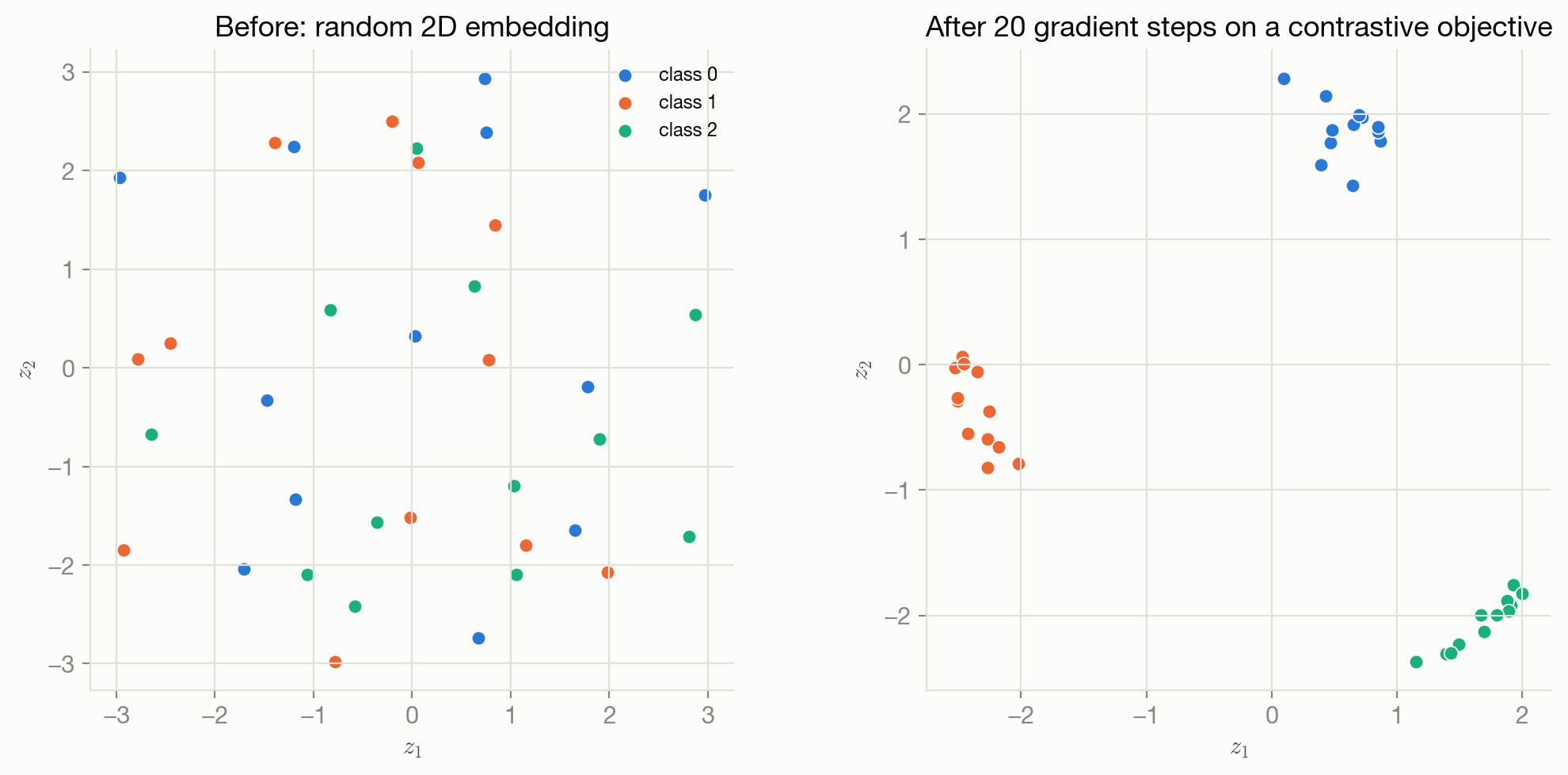
Figure 14.1 makes the geometric goal concrete with an actual (if tiny) computation: points from three synthetic classes, initialized at random positions in 2D with no relationship between position and class, then updated by a small number of explicit gradient steps on a contrastive-style pull/push objective evaluated directly on the point coordinates.
14.6 Interpretation
Minimizing contrastive or triplet loss doesn’t estimate a conditional mean, median, or probability the way the losses in Parts III–V do — it shapes a geometry. What “good” means here is defined entirely in terms of relative distances: same-class points close, different-class points at least a margin apart. Minimizing InfoNCE, read through its cross-entropy reduction, does have the usual NLL interpretation — it pushes the model to assign high probability, under a softmax over the candidate set, to the true match — but because the “candidate set” and hence the classification problem itself changes every time negatives are resampled, there’s no single fixed distribution being fit the way there is for ordinary classification; the model is being asked to solve a new \((K{+}1)\)-way discrimination problem on every example.
14.7 Behavior and edge cases
Contrastive and triplet losses are only informative when the current embedding actually violates the margin — a positive pair that’s already coincident, or a negative pair already separated past \(\mu\), contributes exactly zero gradient. This makes hard-negative mining (deliberately selecting negatives that are currently close to the anchor, so the margin term is active) a practical necessity rather than an optional refinement; without it, most randomly-sampled triplets late in training are already “easy” and contribute nothing. InfoNCE has a related but distinct sensitivity: its softmax denominator sums over \(K\) negatives, so performance depends on both how many negatives are used and how informative they are — too few or too easy negatives make the \((K{+}1)\)-way problem nearly trivial (any embedding solves it, so the gradient carries little information); a large, hard, well-chosen negative pool is what makes InfoNCE-trained representations actually useful.
14.8 Limitations
Contrastive and triplet losses inherit the general heuristic-design weakness Chapter 9 flagged for hinge loss: there is no likelihood being maximized, so no statistical-consistency argument of the Chapter 9 kind transfers automatically, and the margin \(\mu\) is a hyperparameter with no principled default — it has to be tuned to the embedding scale. InfoNCE inherits a different limitation from its construction: the identity of “the positive” is often synthetic (two augmented views, or two sampled examples of the same label) rather than a ground-truth semantic match, so what InfoNCE actually optimizes is invariance to whatever transformation defined the positive pair — a proxy for the representation quality actually wanted, not the goal itself.
14.9 Optimization implications
The margin-based hinge terms in contrastive and triplet loss are non-differentiable at the margin boundary, same as Chapter 9’s hinge, and in practice most of a large batch’s pairs or triplets are inactive at any given step, which is the direct cause of the hard-negative-mining practice described above rather than a separate design issue. InfoNCE’s softmax structure gives it Chapter 6’s usual saturating-gradient behavior, with an added wrinkle: because the denominator sums over \(K\) resampled negatives, larger \(K\) generally gives a better-conditioned, less noisy gradient estimate of the underlying objective, at a direct computational cost — see Chapter 17 for how batch-size and negative-sampling choices more generally trade off against gradient variance.
14.10 Connections
- Chapter 6 supplies the exact categorical cross-entropy formula InfoNCE reduces to — read this chapter’s InfoNCE derivation as a direct application of that one, not a new construction.
- Chapter 9 supplies the margin-based design logic behind both contrastive and triplet loss; the hinge shape here and the hinge shape there exist for the same reason.
- Chapter 11 shares a structural kinship worth noting explicitly: RankNet and this chapter’s objectives all operate on relationships between items (which one outranks which; which pair is a match) rather than on an absolute target for a single item, even though RankNet’s loss is likelihood-derived and contrastive/triplet losses are design choices.
- Chapter 18 can use this chapter as a case study in a loss chosen for the geometry it induces rather than for a statistical guarantee — worth revisiting when working through that chapter’s design questions.