17 Losses and the Optimization Landscape
Every chapter so far has ended with a short “optimization implications” note and moved on, deliberately deferring the details: MSE is a smooth bowl, sigmoid and softmax saturate, hinge has a kink, \(\ell_1\) regularization needs a subgradient. Those notes were promissory. This chapter cashes them in, together, because the comparison is the point: two losses can encode almost the same statistical goal — “penalize the residual,” “penalize a wrong class” — and still produce training runs that behave completely differently, because gradient-based optimization only ever sees a loss’s local shape (its gradient and curvature at the current parameters), not the statistical story that justified it.
17.1 The problem
Everything in Parts II–VIII answered “what does this loss’s minimizer mean?” That question is about where training ends up, assuming it gets there. A separate, equally important question is what happens on the way: how large and how informative the gradient is at a typical point, whether the loss surface is well- or ill-conditioned, whether every point contributes to learning or only some do. Two losses can have the same minimizer’s statistical meaning and radically different answers to these questions.
17.2 Gradient shape: unbounded, saturating, or bounded
A loss’s gradient with respect to its prediction determines how strongly a given example pulls the parameters, and the three losses derived earlier in this book cover three qualitatively different shapes.
Unbounded, linear in the error. Squared error’s gradient with respect to the residual \(r\) is \(r\) itself (Chapter 4) — proportional to how wrong the prediction is, with no ceiling. A point that’s ten times further off contributes ten times the gradient. This is exactly why a single outlier can dominate a minibatch’s gradient (Chapter 5): nothing in the loss’s shape caps its influence.
Saturating. The sigmoid and softmax links behind binary and categorical cross-entropy (Chapter 6) have derivatives that vanish as their argument grows large in magnitude. A prediction that’s confidently and wrong has a large loss value but a small gradient — the direction training most needs to correct is exactly where the signal to correct it is weakest. This is a real, well-documented optimization hazard (it motivates using raw logits rather than post-sigmoid probabilities internally, and is part of why extremely deep or poorly initialized networks can stall early in training).
Bounded / sparse. Hinge loss’s gradient (Chapter 9) is exactly zero for any example with margin greater than 1 — a confidently correct point contributes nothing at all, not even a small pull — and a constant \(\pm1\) for everything else. This is a genuinely different property from saturation: instead of the gradient shrinking smoothly, it switches off completely, meaning only a subset of training points (the “support vectors,” in the SVM literature this loss comes from) ever influence the gradient at a given step. Huber’s gradient (Chapter 5) is the deliberately engineered middle ground: linear (informative) near zero, capped at \(\pm\delta\) beyond it — bounded like hinge, but never exactly zero.
17.3 Curvature and conditioning
Curvature — the loss’s second derivative — determines how a fixed step size behaves, and here squared error and absolute error are opposites. MSE’s curvature is the constant \(1\) everywhere (a perfect, unchanging quadratic bowl), which is exactly what makes it so well-behaved for gradient descent and Newton-type methods alike: the local quadratic approximation a second-order method builds is the true function, everywhere, not just near the optimum. MAE’s curvature is \(0\) almost everywhere (the loss is locally linear away from zero) and undefined exactly at the residual where it matters. A method that relies on curvature information — Newton’s method, natural gradient, many quasi-Newton schemes — gets essentially nothing useful from MAE’s second derivative. Huber again splits the difference: curvature \(1\) within \(\delta\) of the target, \(0\) beyond it, so a point far from being fit correctly is optimized using first-order information only, while a point close to converged benefits from full second-order behavior.
None of this is a statement about which loss is “better” — Chapters 4, 5, and 8 already settled what each one’s minimizer means, on entirely separate grounds. This is a second, independent axis: given that you’ve chosen a loss for its statistical properties, what does that same choice cost or buy you computationally?
17.4 Smoothness: where the kinks live, and why they’re not accidents
Three real non-differentiabilities appear earlier in this book, and all three are the source of the property that made that loss useful, not an unfortunate side effect: MAE’s kink at \(r=0\) (Chapter 5) is exactly what makes its minimizer a median rather than a mean; the \(\ell_1\) regularizer’s kink at \(w=0\) (Chapter 3) is exactly what lets MAP estimation land on exactly zero and produce sparsity; hinge’s kink at margin \(=1\) (Chapter 9) is exactly what makes only a subset of points support vectors. Plain gradient descent doesn’t strictly require differentiability (a subgradient suffices almost everywhere), but methods that assume smoothness — line searches that use curvature, many second-order and quasi-Newton methods — need modification (subgradient methods, proximal operators) at these points. The general playbook for this is optimization-lab’s territory, not this book’s; the point here is narrower and specific to loss design: a kink you introduce on purpose to get a statistical property is a kink you’re also choosing to hand your optimizer.
17.5 A concrete comparison
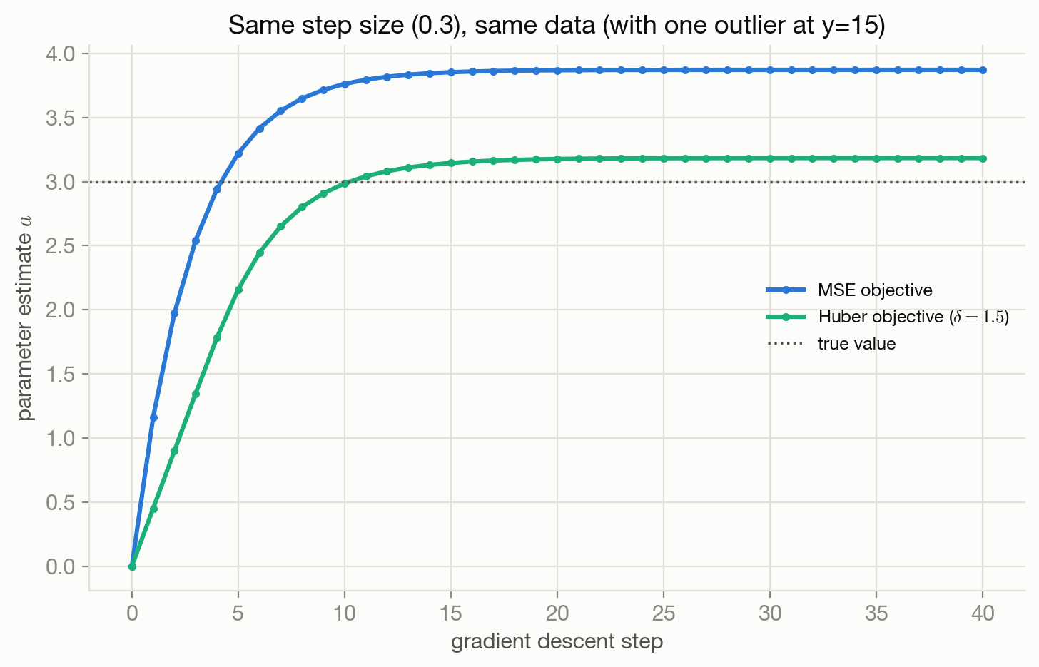
Figure 17.1 runs plain gradient descent, same fixed step size, same dataset (14 points near a true value of 3, plus one strong outlier at 15), on MSE and on Huber. Both trajectories converge smoothly — neither loss is so ill-conditioned here that it oscillates or diverges — but they converge to visibly different places and along visibly different paths. MSE’s gradient at the starting point is dominated by the outlier (its contribution is proportional to its own huge residual), so the trajectory initially races toward a value inflated by that single point before slowly settling at the outlier-pulled mean, \(3.87\). Huber’s gradient contribution from that same point is capped, so its pull is present but never dominant throughout, and the trajectory settles at \(3.19\), much closer to the true value of \(3\). This is the same robustness story as Chapter 5’s outlier-fitting figure, now viewed frame-by-frame rather than only at convergence: the bounded-gradient property isn’t just a fact about the final answer, it’s visible in every single step along the way.
17.6 What this chapter doesn’t replace
This chapter connects loss shape to optimization behavior — it does not develop optimization theory itself. Line search, momentum, adaptive per-parameter step sizes (Adam and relatives), condition-number bounds on convergence rate, and the general theory of convex and non-convex optimization are the proper subject of optimization-lab, which this book leans on rather than duplicates. What belongs here, and only here, is the observation that precedes all of that machinery: before asking which optimizer to use, it’s worth knowing what your loss’s own gradient and curvature already look like, because no optimizer can add back second-order information a loss doesn’t have, or undo the influence an unbounded gradient hands to a single bad data point.
17.7 Connections
- Chapter 4 and 5 supply the MSE/MAE/Huber gradient and curvature comparison this chapter makes explicit and visual.
- Chapter 6 flagged sigmoid and softmax saturation as a deferred optimization concern — this is where that’s picked back up.
- Chapter 9 and 3 are where hinge’s and \(\ell_1\)’s kinks were first introduced as features, not bugs — this chapter names the optimization price of that choice explicitly.
- Chapter 18 puts “what do its gradients and curvature look like?” directly into its checklist for designing a new loss — this chapter is the worked background for that step.