7 Entropy, Cross-Entropy, and KL Divergence
Chapter 6 derived cross-entropy as a likelihood, without ever mentioning information theory. That derivation is complete and correct on its own terms — but “cross-entropy” is also the name of a specific information- theoretic quantity, and the fact that classification’s NLL and that quantity are the same formula is not a coincidence worth leaving unexplained. This chapter builds the information-theoretic apparatus from its own definitions, proves the exact relationship to KL divergence, and is deliberately careful about a distinction that gets blurred constantly: cross-entropy and KL divergence share a minimizer, but they are not interchangeable numbers, and conflating them is one of the easiest ways to misread this part of the literature.
7.1 The problem
Given two distributions over the same outcomes — a true or target distribution \(P\) and a model’s distribution \(Q\) — how much does \(Q\) cost you, in a precise, quantifiable sense, when the world actually behaves according to \(P\)? Answering this rigorously is what makes it possible to say precisely what classification’s cross-entropy loss is measuring, beyond “a formula that happens to match the Bernoulli/categorical NLL.”
7.2 Derivation
Entropy: the cost of describing \(P\) optimally
Shannon’s entropy (Shannon 1948) quantifies the intrinsic uncertainty in a distribution \(P\) over a discrete set of outcomes:
\[ H(P) = -\sum_x P(x)\log P(x) \]
The standard operational reading (Cover and Thomas give the full derivation (Cover and Thomas 2006)): if you had to design an optimal code for outcomes drawn from \(P\) — short codewords for likely outcomes, long ones for unlikely — the expected codeword length of the best possible code is \(H(P)\) (in bits, using \(\log_2\); in nats, using \(\log_e\) as this book does throughout). \(H(P)\) is a property of \(P\) alone; it doesn’t reference any model.
Cross-entropy: the cost of using the wrong code
Now suppose the code was designed assuming outcomes are drawn from \(Q\), but they’re actually drawn from \(P\):
\[ H(P,Q) = -\sum_x P(x)\log Q(x) \]
\(H(P,Q)\) is the expected codeword length of that (mismatched) code, under the true distribution \(P\). Using a code optimized for the wrong distribution can only cost more, never less, than using the right one — which is the content of the identity below.
KL divergence and the decomposition
\[ D_{\mathrm{KL}}(P\,\|\,Q) = \sum_x P(x)\log\frac{P(x)}{Q(x)} \]
introduced by Kullback and Leibler as a measure of how distinguishable two distributions are (Kullback and Leibler 1951). Expand the definition and split the log of a ratio into a difference of logs:
\[ D_{\mathrm{KL}}(P\|Q) = \sum_x P(x)\big[\log P(x) - \log Q(x)\big] = -H(P) - \sum_x P(x)\log Q(x) = H(P,Q) - H(P). \]
Rearranged:
\[ H(P,Q) = H(P) + D_{\mathrm{KL}}(P\,\|\,Q). \]
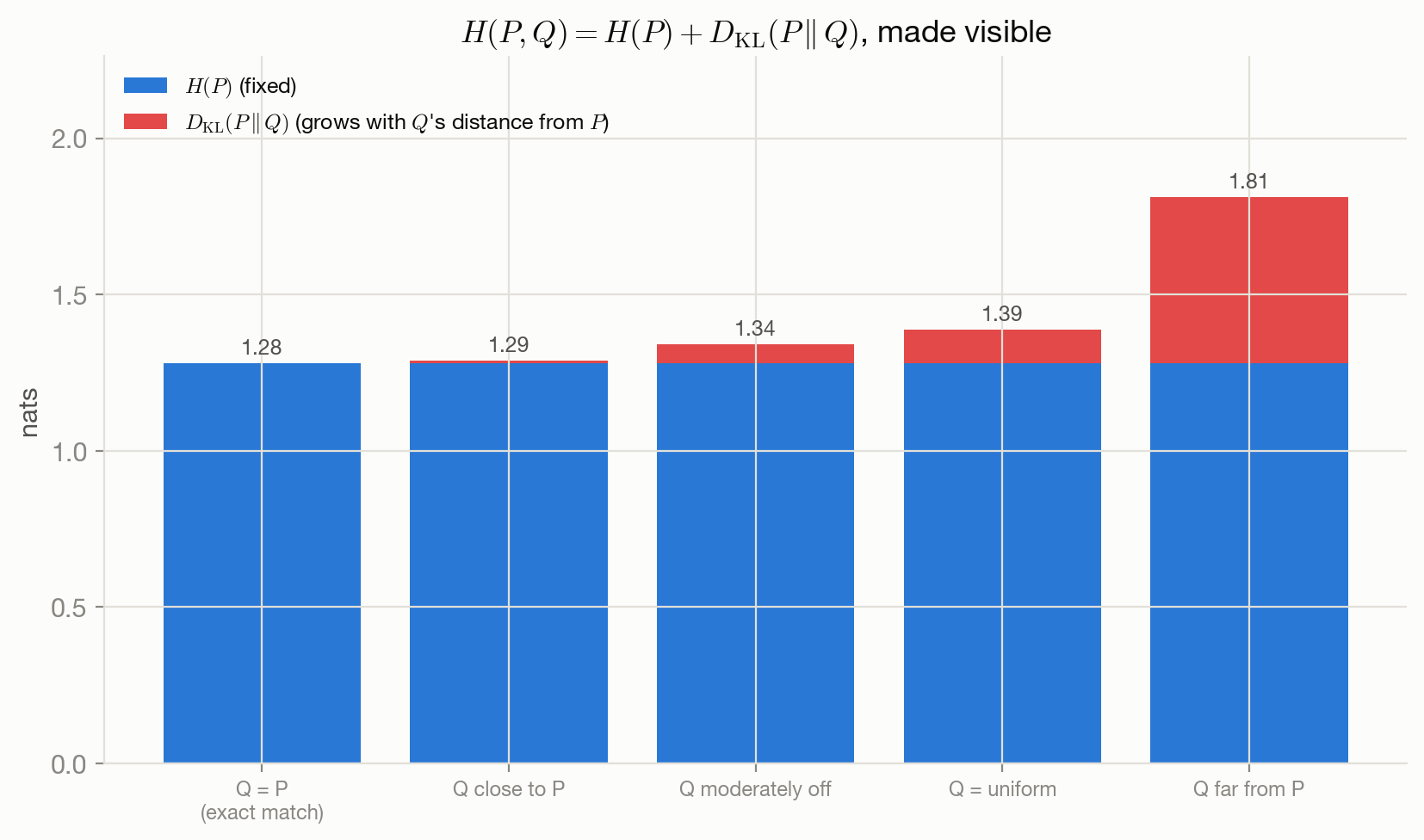
In the coding-cost language above: the extra expected cost of the mismatched code (\(H(P,Q)\)) equals the unavoidable minimum cost (\(H(P)\)) plus exactly the extra cost attributable to the mismatch itself (\(D_{\mathrm{KL}}(P\|Q)\), which is \(\ge 0\) always, with equality only when \(Q=P\) almost everywhere — a fact this chapter states without proof; see (Cover and Thomas 2006)). Figure 7.1 makes the decomposition visible directly: for a fixed target \(P\) over four outcomes and several choices of \(Q\) ranging from an exact match to far off, every bar’s total height (\(H(P,Q)\)) splits cleanly into a constant bottom segment (\(H(P)\)) and a growing top segment (\(D_{\mathrm{KL}}(P\|Q)\)).
Reconnecting to Chapter 6
In classification, \(P\) is the target distribution over classes — often one-hot, \(P(c)=1\) at the true class and \(0\) elsewhere — and \(Q=Q_\theta\) is the model’s predicted distribution. Because \(P\) doesn’t depend on \(\theta\), \(H(P)\) is a fixed constant with respect to \(\theta\), so
\[ \arg\min_\theta H(P, Q_\theta) = \arg\min_\theta D_{\mathrm{KL}}(P\,\|\,Q_\theta) \]
— minimizing cross-entropy and minimizing KL divergence from the fixed target to the model pick out exactly the same \(\theta\). This is the precise sense in which Chapter 6’s cross-entropy loss “is” a KL-divergence minimization, and it’s worth being exact about what that sentence does and doesn’t claim.
7.3 The one-hot special case, and why it isn’t the general case
When \(P\) is one-hot, \(H(P) = -1\cdot\log 1 - \sum_{\text{other } x} 0\cdot\log 0 = 0\) (using the standard convention \(0\log 0 = 0\)), so \(H(P,Q_\theta) = D_{\mathrm{KL}}(P\|Q_\theta)\) exactly — not just up to a constant, but as equal numbers, because the constant happens to be zero. This special case is common enough in ordinary hard-label classification that it’s easy to walk away believing cross-entropy and KL divergence are simply the same thing. They are not: as soon as \(P\) isn’t one-hot — label smoothing (spreading a little probability mass off the true class on purpose), soft targets from knowledge distillation, or genuine soft labels from multiple human annotators — \(H(P) > 0\), and cross-entropy and KL divergence become different numbers that happen to still share a minimizer only as long as \(P\) itself stays fixed while \(\theta\) varies. If \(P\) is also allowed to change (comparing across different label distributions, for instance), even the shared-minimizer property no longer applies.
7.4 Interpretation
\(D_{\mathrm{KL}}(P\|Q)\) answers “how distinguishable is \(Q\) from \(P\),” weighted from \(P\)’s perspective; \(H(P,Q)\) answers “what does it cost, in expectation under \(P\), to use \(Q\)’s code.” Training a classifier by cross-entropy is, exactly, training it to make its predicted distribution as close to indistinguishable from the target distribution as the \(H(P)\)-independent part of that cost allows.
7.5 Behavior and edge cases
\(D_{\mathrm{KL}}(P\|Q)\) is asymmetric: \(D_{\mathrm{KL}}(P\|Q) \neq D_{\mathrm{KL}}(Q\|P)\) in general, and it is undefined (or infinite) wherever \(P(x)>0\) but \(Q(x)=0\) — the mismatched code has literally no codeword for an outcome the true distribution says can happen. This directly explains Chapter 6’s observation that assigning exactly zero probability to the true class is catastrophic: it’s not a large KL divergence, it’s an undefined one.
7.6 Limitations
None of this apparatus says anything about how to estimate \(Q_\theta\) or how many samples are needed to estimate \(H(P,Q)\) accurately from data — those are separate statistical questions the pure information-theoretic identity above is silent on.
7.7 Connections
- Chapter 6 is the loss this chapter formalizes; read them as a pair.
- Chapter 2 placed NLL, cross-entropy, and (implicitly) KL divergence in relation to each other for the first time — this chapter is where that triad becomes precise rather than suggestive.
- Chapter 11 and 12 reuse this exact log-probability-of-the-truth machinery for pairwise preferences and full permutations instead of classes.
- Chapter 14’s InfoNCE objective has a mutual-information reading that traces directly back to the KL machinery built here.