2 From Probability Models to Objectives
Chapter 1 left a gap on purpose: a loss \(\ell(\theta;x,y)\) turns a prediction error into a number, but nothing so far says which turning rule to use. This chapter supplies the first, and most important, principled answer. It doesn’t start from a loss at all — it starts from reinterpreting what the model \(f_\theta\) is doing, and a specific, non-arbitrary loss falls out of that reinterpretation as a consequence, not a choice.
2.1 The problem
Instead of asking \(f_\theta\) to output a single number \(\hat y\) and penalizing its distance from \(y\), suppose \(f_\theta\) is asked to output a full probability distribution over possible targets: \(p(y \mid x; \theta)\). A linear regression model predicting a single number is really claiming “\(y\) is near this value”; a model that instead outputs \(p(y\mid x;\theta) = \mathcal{N}(f_\theta(x), \sigma^2)\) is making a sharper, falsifiable claim: it says exactly how probable every possible \(y\) is, not just which one is likeliest. The question this chapter answers is: given that a model makes probabilistic claims like this, what does it mean to train it — and does that training procedure look like empirical risk minimization from Chapter 1?
2.2 Assumptions
Two assumptions carry the whole chapter, and it’s worth stating them as assumptions rather than facts, because Chapter 3 will spend real effort on what happens when they’re wrong.
- The model is a genuine conditional distribution. \(p(y\mid x;\theta)\) is a properly normalized probability (density for continuous \(y\), mass for discrete \(y\)) over \(\mathcal{Y}\), for every \(x\) and every \(\theta\).
- The data is i.i.d. given the model. \((x_1,y_1),\dots,(x_n,y_n)\) are drawn independently, so the probability of the dataset under the model factors into a product of per-example probabilities.
2.3 Derivation
The likelihood
Define the likelihood as the probability the model assigns to the data actually observed, viewed as a function of \(\theta\) with the data held fixed:
\[ \mathcal{L}(\theta) = p(D \mid \theta) = \prod_{i=1}^n p(y_i \mid x_i; \theta). \]
The product is a direct consequence of assumption 2 (independence); nothing more subtle is happening in this step. \(\mathcal{L}(\theta)\) answers “how probable would this exact dataset have been, if \(\theta\) were the true parameter?” — a question about \(\theta\), even though it’s built entirely from a probability statement about data. This is the distinction the notation appendix flags with the \(\ell\) vs. \(\mathcal{L}\) split: \(\mathcal{L}(\theta)\) is not a loss yet, and it is not a probability distribution over \(\theta\) — it doesn’t have to integrate to 1 over \(\theta\), and usually doesn’t.
Maximum likelihood estimation (MLE), formalized by Fisher (Fisher 1922), is the principle of choosing \(\theta\) to make the observed data as probable as possible under the model:
\[ \hat\theta_{\mathrm{MLE}} = \arg\max_\theta \mathcal{L}(\theta). \]
Why the logarithm
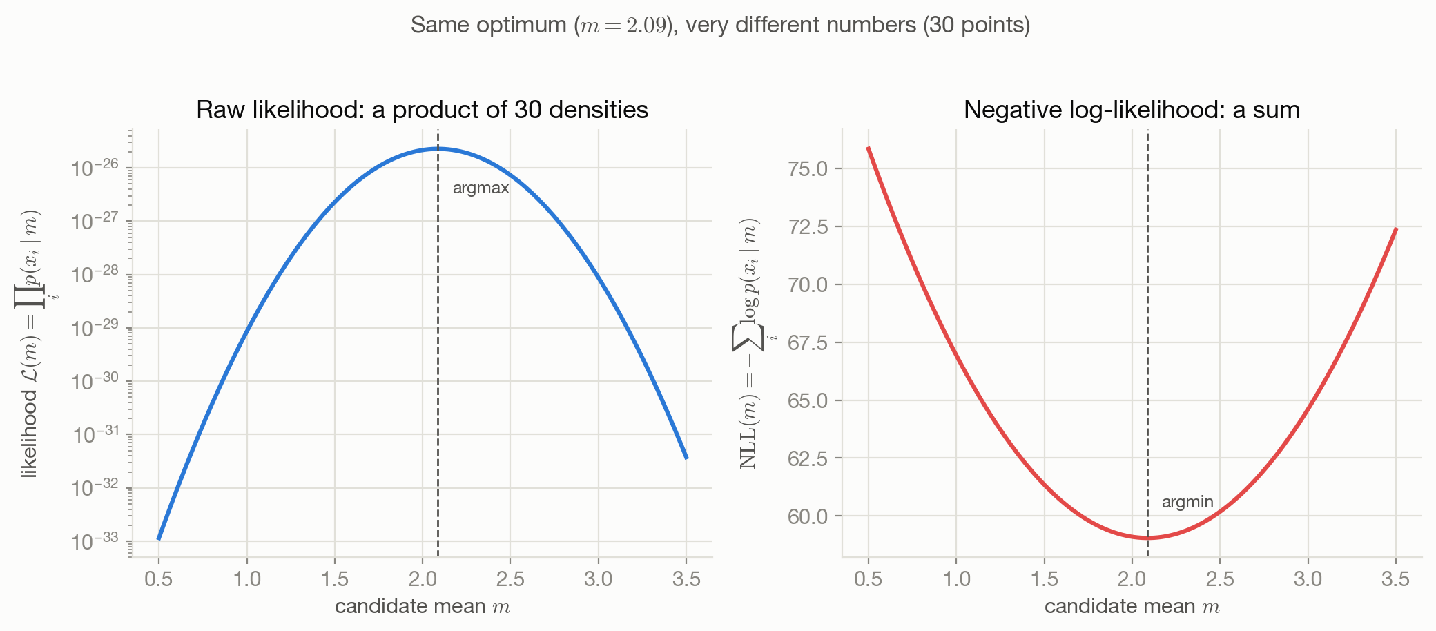
\(\mathcal{L}(\theta)\) is a product of up to millions of terms, each a probability — a number no larger than 1, usually much smaller. This is a genuine numerical problem, not a stylistic one: the companion script behind Figure 2.1 finds that even the best-fitting mean for just \(n=30\) Gaussian-distributed points already gives a raw likelihood around \(2\times10^{-26}\), and that this only gets worse with more data — by \(n=800\) points, the true best-fitting likelihood underflows to exactly \(0.0\) in 64-bit floating point, even though the data and the model are both completely well-behaved. Whatever function is used to find \(\hat\theta\) needs to avoid ever materializing \(\mathcal{L}(\theta)\) as a raw number.
The logarithm fixes this and does one more useful thing at the same time. Because \(\log\) is strictly increasing, it doesn’t change where a function is maximized:
\[ \arg\max_\theta \mathcal{L}(\theta) = \arg\max_\theta \log\mathcal{L}(\theta). \]
And because \(\log\) turns products into sums,
\[ \log \mathcal{L}(\theta) = \log\prod_{i=1}^n p(y_i\mid x_i;\theta) = \sum_{i=1}^n \log p(y_i \mid x_i;\theta). \]
This sum form has a second, independent benefit beyond numerical range: its gradient with respect to \(\theta\) is a sum of per-example gradients, \(\nabla_\theta \log\mathcal{L}(\theta) = \sum_i \nabla_\theta \log p(y_i\mid x_i;\theta)\), which is precisely what makes minibatch stochastic gradient descent a valid approximation — a random subset of the sum is an unbiased estimate of the whole sum. None of this would be available from the raw product.
From maximizing to minimizing
Everything built so far is still a maximization. Chapter 1 defined risk as something to be minimized, matching the near-universal convention that training code minimizes a loss. One more step reconciles them: negating a function turns its maximizer into its minimizer, so
\[ \arg\max_\theta \mathcal{L}(\theta) = \arg\max_\theta \log\mathcal{L}(\theta) = \arg\min_\theta \Big(-\log \mathcal{L}(\theta)\Big). \]
Figure 2.1 puts the whole transformation on screen at once, fitting a single Gaussian mean to \(n=30\) points: the raw likelihood on the left, spanning dozens of orders of magnitude and numerically unusable, and its negative log — the quantity this section just arrived at — on the right, an ordinarily-scaled, convex curve whose minimum sits at exactly the same parameter value as the raw likelihood’s maximum. Neither the log nor the negation moves the optimum; together they just make the function usable.
2.4 The resulting objective
\[ \mathrm{NLL}(\theta) = -\log\mathcal{L}(\theta) = -\sum_{i=1}^n \log p(y_i \mid x_i; \theta). \]
This isn’t a loss chosen for convenience and later found to have a probabilistic flavor — it’s the direct, forced consequence of (a) treating \(f_\theta\) as defining a distribution and (b) wanting to make the observed data as probable as possible. Every specific loss derived in Parts III and IV of this book (squared error, absolute error, binary and categorical cross-entropy) is this exact same NLL, specialized to a particular choice of \(p(y\mid x;\theta)\) — not a separately invented formula that happens to resemble it.
2.5 Interpretation
Define \(\ell(\theta;x,y) := -\log p(y\mid x;\theta)\). Then \(\mathrm{NLL}(\theta) = \sum_i \ell(\theta; x_i, y_i) = n\,\hat R(\theta)\) — minimizing NLL is exactly empirical risk minimization from Chapter 1, under the specific per-example loss “negative log-probability the model assigned to what actually happened.” This is the payoff of the whole construction: instead of inventing \(\ell\) by intuition, a probabilistic assumption about \(y\) determines \(\ell\) uniquely.
2.6 Behavior and edge cases
\(-\log p(y\mid x;\theta)\) is \(0\) only when \(p(y\mid x;\theta)=1\) — total certainty, exactly matched to what happened — and grows without bound as \(p(y\mid x;\theta) \to 0\). A model that assigns near-zero probability to the outcome that actually occurred is punished arbitrarily severely, not mildly; a model that hedges (\(p\) close to uniform) pays a moderate, bounded cost. This asymmetry — confident-and-wrong is much worse than uncertain-and-wrong — turns out to be exactly the shape that makes cross-entropy (Chapter 6) work as a classification loss, and it is a direct, mechanical consequence of the logarithm, not a separately chosen design feature.
2.7 Limitations
NLL is only as meaningful as the distributional assumption it’s built on. If \(p(y\mid x;\theta)\) is misspecified — the true conditional distribution of \(Y\) isn’t actually in the assumed family — \(\hat\theta_{\mathrm{MLE}}\) still exists and training still runs, but it no longer has the statistical guarantees (consistency, asymptotic efficiency) that motivate MLE in the first place. And MLE, as derived here, returns a single point \(\hat\theta\); it says nothing about how much that estimate should be trusted, which is exactly the gap Chapter 3’s move to a posterior over \(\theta\) addresses.
2.8 Optimization implications
The sum structure derived above — not assumed, but a direct consequence of independence plus the log — is what makes NLL tractable at scale: its gradient is additive over examples, enabling stochastic and minibatch optimization. What the curvature of NLL looks like depends entirely on which distribution was assumed (Gaussian NLL is quadratic and well-conditioned; categorical NLL after a softmax has flatter regions at extreme logits) — that comparison is deferred to Chapter 17, once several concrete instances exist to compare.
2.9 Connections
- Chapter 1 supplies the vocabulary this chapter closes the loop on: NLL is not a new kind of object, it’s a specific, principled instance of the per-example loss \(\ell\) and empirical risk \(\hat R\) already defined there.
- Chapter 3 is the direct continuation: it names \(\hat\theta_{\mathrm{MLE}}\) explicitly and asks what changes when a prior over \(\theta\) is added, turning MLE into MAP.
- Chapters 4 through 7 are this chapter’s payoff: each picks a specific \(p(y\mid x;\theta)\) — Gaussian, Laplace, Bernoulli, categorical — and works out exactly what \(\mathrm{NLL}(\theta)\) becomes.
- Chapter 15 applies this exact derivation — likelihood, product over i.i.d.-ish units, log, sum — to sequences of tokens instead of independent examples.