10 Why Ranking Needs Different Objectives
Every objective so far has scored a single prediction against a single target: one \(\hat y\) against one \(y\). Ranking breaks that mold. The target is now a full ordering over a set of items — search results for a query, candidates for a recommendation slot, completions for a prompt — and what makes a ranking “good” is a property of the whole list, not of any one item’s prediction in isolation. Two lists can agree on every individual item’s estimated relevance and still be scored very differently on ranking quality, because what matters is which items end up on top. This part of the book (four chapters) asks where ranking objectives actually come from, and this chapter sets up the vocabulary the rest reuses.
10.1 The problem
Given a query or context \(x\) and a set of candidate items \(\{x_1,\dots,x_n\}\) with an observed relevance ordering \(y_1 > y_2 > \cdots\) (or graded relevance scores), produce scores \(s_i = f_\theta(x_i)\) whose sort order matches the target ordering as closely as possible, with an emphasis on getting the top of the list right — a search engine that nails position 1 but shuffles positions 40–50 is doing its job; one that does the reverse is not.
Three strategies show up repeatedly, and naming them now makes the next three chapters easier to place:
Pointwise. Treat each item’s relevance as an independent regression or classification target and reuse a loss from Chapters 4–9 per item. This is simple and reuses everything already built, but it optimizes each item’s score in isolation — it has no way to express “getting item 1 right matters more than item 40,” because it never compares items to each other at all.
Pairwise. Compare items two at a time: does the model correctly order each observed pair? Chapter 11 derives RankNet, the canonical pairwise objective.
Listwise. Model the probability of an entire observed ranking at once. Chapter 12 derives ListMLE, built from exactly this idea.
10.2 Ranking metrics
Ranking quality is normally measured with metrics that weight position explicitly. For a ranked list with relevance grades \(\mathrm{rel}_1, \mathrm{rel}_2,\dots\) (in the order the model produced), discounted cumulative gain is
\[ \mathrm{DCG@k} = \sum_{i=1}^{k} \frac{2^{\mathrm{rel}_i}-1}{\log_2(i+1)}, \]
which rewards high relevance and discounts it logarithmically the further down the list it appears — a highly relevant item at position 1 contributes far more than the same item at position 20. Normalized DCG, \(\mathrm{NDCG@k} = \mathrm{DCG@k} / \mathrm{IDCG@k}\), divides by the DCG of the ideal (perfectly sorted) ordering, rescaling the metric to \([0,1]\) so it’s comparable across queries with different numbers of relevant items (Järvelin and Kekäläinen 2002). Mean reciprocal rank (MRR) instead scores only the position of the first relevant result, \(1/\mathrm{rank}_{\text{first}}\), appropriate when only one correct answer is expected. Mean average precision (MAP) averages precision computed at every position a relevant item appears, appropriate for multiple binary-relevant results.
10.3 Why these metrics resist direct optimization
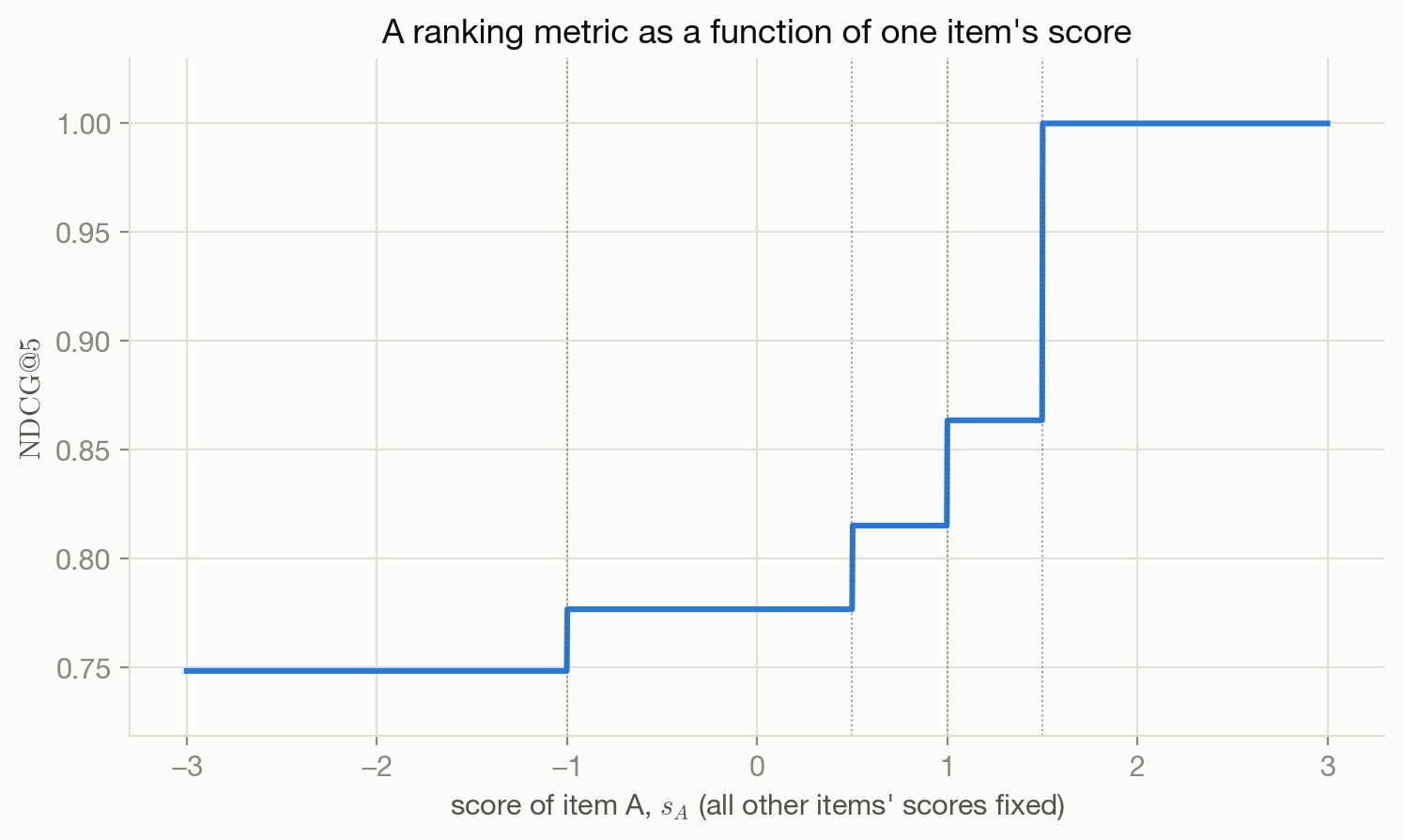
Every metric above is a function of the rank positions the scores induce — which is to say, a function of \(\mathrm{argsort}(s_1,\dots,s_n)\). That sort order changes only at the discrete moments when two items’ scores cross; anywhere else, nudging a score slightly changes nothing about the metric at all. Formally, \(\mathrm{argsort}\) is piecewise-constant in the scores, so any metric built from rank position has zero gradient with respect to the scores almost everywhere, and an undefined one exactly where two scores tie — precisely the ties where nudging should matter most.
Figure 10.1 makes this concrete: fixing four items’ scores and a set of relevance grades, and sweeping a fifth item’s score continuously, \(\mathrm{NDCG@5}\) doesn’t move smoothly at all — it sits flat, then jumps discontinuously the instant the swept score crosses another item’s fixed score, four times across the sweep, with zero slope everywhere else. A gradient-based optimizer looking at this function has nothing to follow almost everywhere it might start.
10.4 The recurring pattern: metric, loss, surrogate
This is the same shape of problem Chapter 9 ran into with 0–1 classification loss, now one level up: the quantity that actually defines success (0–1 accuracy there, NDCG/MRR/MAP here) is exactly the quantity that’s hardest to differentiate, precisely because “hardest decisions” tend to be the discrete, threshold-crossing kind. The response is the same each time, and it breaks down into five questions worth asking in order, every time this shape of problem shows up again:
- What property of a good outcome is actually wanted? (Here: getting the top of a ranked list right.)
- What metric captures it? (NDCG, MRR, or MAP, depending on the task.)
- Why can’t that metric be optimized directly? (It’s a function of \(\mathrm{argsort}\) — piecewise-constant, zero gradient almost everywhere.)
- What surrogate captures the desired behavior anyway, even though it isn’t the metric itself? (Chapter 11 and Chapter 12 build two different, principled surrogates this way; Chapter 13 goes further and builds a surrogate that’s explicitly aware of which metric it’s standing in for.)
- What assumptions does that surrogate introduce, and how well do they actually track the metric it’s standing in for?
Keeping “metric,” “loss,” and “surrogate” as three distinct words for three distinct things — not synonyms — is exactly the discipline Chapter 18’s design recipe leans on for problems well outside ranking.
10.5 Connections
- Chapter 9 established the metric/loss/surrogate pattern for classification (0–1 loss vs. hinge/logistic); this chapter is the same pattern one level up, for whole orderings instead of single labels.
- Chapter 11 and Chapter 12 are the two surrogate families this chapter sets up — pairwise and listwise, respectively.
- Chapter 13 returns to attacking NDCG more directly, once RankNet and ListMLE are both on the table to compare against.
- Chapter 18’s recipe for designing a new loss explicitly reuses the metric → loss → surrogate reasoning pattern named here, applied to an arbitrary new problem.