3 Supervised Learning
Most of applied machine learning, in practice, reduces to one question: given a pile of past examples where you knew the right answer, can you build something that guesses the right answer for a new example you haven’t seen? That is supervised learning. You have inputs \(x\) — a user’s clickstream, a patient’s lab values, a photo, a sentence — and a target \(y\) that you observed for past cases — did they churn, did they have the disease, what’s in the photo, what’s the sentiment. Supervised learning fits a function \(f\) so that \(f(x) \approx y\) on the examples you have, in a way that generalizes to examples you don’t. Nearly every classifier, regressor, ranker, and risk score running in production today is a descendant of this idea, and most of the concepts that make deep learning work — loss functions, regularization, generalization gaps, calibration — are inherited directly from this foundational setting rather than invented for neural networks.
The reason supervised learning is worth understanding carefully, rather than just calling .fit(), is that almost every practical failure in applied ML traces back to a violation of one of its core assumptions: that the labels are a faithful measurement of what you actually care about, that future data looks statistically like past data, and that a model which fits the training examples well will keep working on new ones. None of those are automatic.
3.1 How it works
Empirical risk minimization
Formally, supervised learning assumes there is some (unknown, possibly noisy) process generating pairs \((x, y)\) according to a joint distribution \(p(x, y)\). What you actually want is a function \(f\) that minimizes the expected loss over that whole distribution — the risk:
\[ R(f) = \mathbb{E}_{(x,y) \sim p}\big[\, \ell(f(x), y) \,\big] \]
where \(\ell\) is a loss function measuring how bad a prediction is (squared error for regression, cross-entropy for classification, and so on). The problem is that you don’t have access to \(p(x, y)\) — you only have a finite sample of \(n\) examples drawn from it. So instead you minimize the empirical risk, the average loss over the data you actually have:
\[ \hat{R}(f) = \frac{1}{n} \sum_{i=1}^{n} \ell(f(x_i), y_i) \]
This substitution — optimizing the empirical average in place of the true expectation — is called empirical risk minimization (ERM), and it is the mechanical core of essentially all of supervised learning: gradient descent on a training set, fitting a decision tree by minimizing impurity, fitting a GLM by maximum likelihood are all instances of ERM with a particular choice of \(f\)’s functional form and \(\ell\)’s shape. ERM works because, under mild conditions (i.i.d. sampling, a hypothesis class that isn’t too flexible relative to \(n\)), the law of large numbers guarantees \(\hat{R}(f)\) converges to \(R(f)\) as \(n\) grows. But for any finite \(n\), driving \(\hat{R}(f)\) to zero does not guarantee \(R(f)\) is small — a function can memorize the training sample perfectly while representing \(p(x,y)\) terribly. That gap between minimizing the thing you can measure (training loss) and the thing you actually want (generalization) is the central tension of the whole field.
Why the bias-variance tradeoff exists
The gap between training and test performance has a clean decomposition for squared-error regression, and it’s worth deriving because the same underlying force operates in classification and deep learning even where the tidy algebra doesn’t. Suppose the true relationship is \(y = g(x) + \varepsilon\) where \(\varepsilon\) has mean zero and variance \(\sigma^2\), and we fit \(\hat{f}\) on a random training set \(D\). For a fixed test point \(x\), the expected squared error, averaged over both the noise and the randomness of which training set we happened to draw, decomposes as:
\[ \mathbb{E}_D\big[(y - \hat{f}_D(x))^2\big] = \underbrace{\big(g(x) - \mathbb{E}_D[\hat{f}_D(x)]\big)^2}_{\text{bias}^2} + \underbrace{\mathrm{Var}_D\big[\hat{f}_D(x)\big]}_{\text{variance}} + \underbrace{\sigma^2}_{\text{irreducible noise}} \]
Bias is the error from the model’s functional form being fundamentally too rigid to represent \(g\) — a straight line fit to a curve is biased no matter how much data you feed it. Variance is the error from the model being so flexible that it fits the idiosyncratic noise of whatever particular training sample it happened to see — retrain on a different sample of the same size and you’d get a noticeably different function. These two terms move in opposite directions as you change model complexity: a rigid model (low polynomial degree, shallow tree, strong regularization) has high bias but low variance across resamples; a flexible model (high-degree polynomial, deep unpruned tree, weak regularization) has low bias but high variance. Total expected error is minimized somewhere in between, not at either extreme. This is not a rule of thumb — it’s an algebraic identity, and it’s why “just use the most expressive model” is not a strategy: expressiveness only helps up to the point where variance starts to dominate.
Figure 3.1 makes this concrete on a toy 1D regression problem. Twenty-five noisy points are generated from a smooth nonlinear function, and polynomials of increasing degree are fit to them.
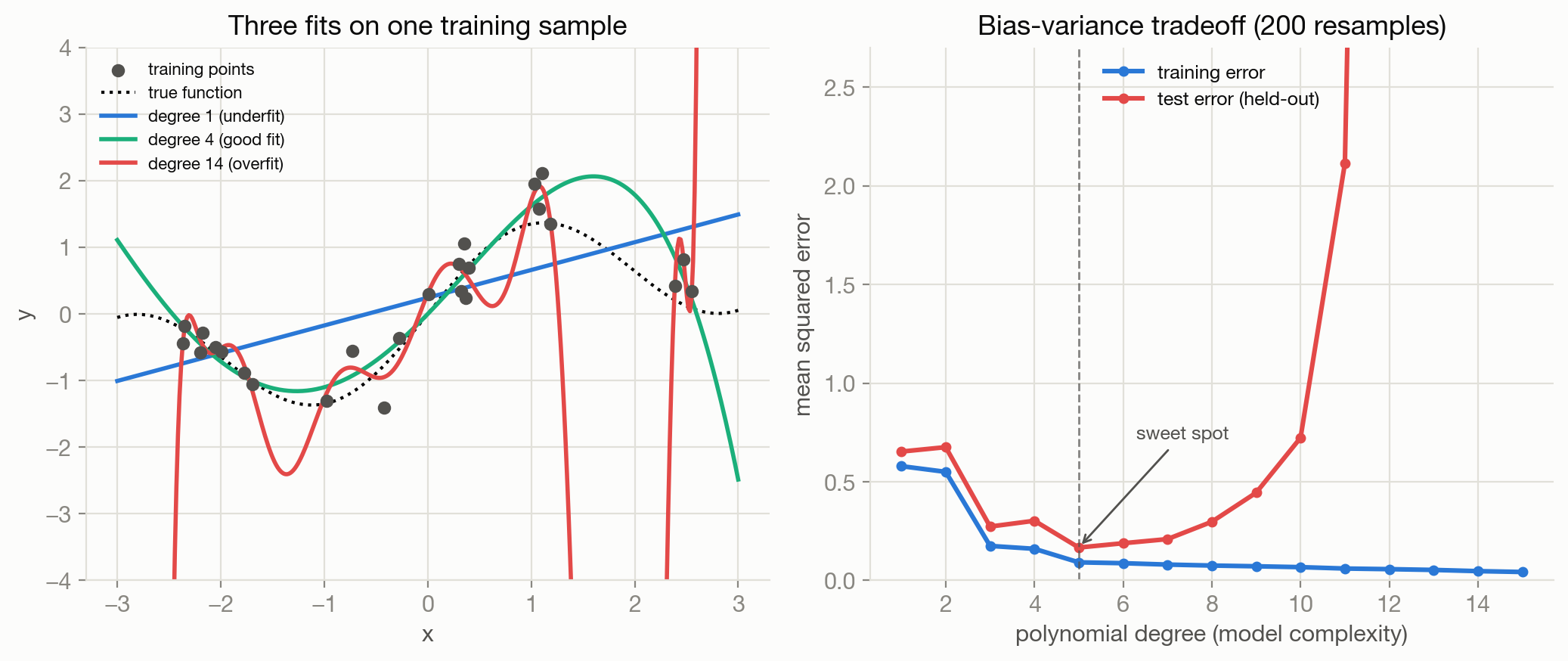
Notice the specific asymmetry in the right panel: training error keeps improving (or staying flat) as complexity increases — a strictly more expressive hypothesis class can always match the training sample at least as well — but test error is U-shaped. The widening gap between the two curves at high degree is exactly the variance term; the height of the test curve at low degree, where the two curves nearly coincide, is dominated by bias. This is also the picture to have in mind for any model family, not just polynomials: model depth in a tree, hidden width in a neural net, \(k\) in k-NN, and the inverse of a regularization strength all trace out the same shape.
Loss functions encode what “wrong” means
The choice of \(\ell\) is not a technicality — it defines what the model is actually being optimized to get right. Squared error \((f(x) - y)^2\) penalizes large errors quadratically and its minimizer, in expectation, is the conditional mean \(\mathbb{E}[y \mid x]\); it is the right choice when big misses are disproportionately bad and the target is continuous. Absolute error \(|f(x) - y|\) is minimized by the conditional median, and is more robust to outliers because it doesn’t square large residuals. For binary classification, cross-entropy loss \(-\big[y \log \hat{p} + (1-y)\log(1-\hat{p})\big]\) is minimized by the true conditional probability \(p(y=1\mid x)\), which is exactly why models trained with cross-entropy (logistic regression, most neural classifiers) produce outputs that can be interpreted as probabilities — while a model trained to minimize 0/1 accuracy directly has no such guarantee, and accuracy isn’t even a differentiable target for gradient-based training. Picking a loss is picking a definition of “the best possible prediction given the information in \(x\),” and that definition should match what the downstream decision actually needs (a point estimate, a probability, a quantile, a ranking).
Regularization is a prior, not a penalty
Regularization is usually introduced as “add a penalty term to discourage large weights,” which is true but obscures why that helps. Consider ridge regression, which minimizes:
\[ \hat{R}_{\text{ridge}}(\beta) = \sum_{i=1}^n (y_i - x_i^\top \beta)^2 + \lambda \|\beta\|_2^2 \]
This is exactly the negative log-posterior (up to a constant) you’d get from placing an independent Gaussian prior \(\beta_j \sim \mathcal{N}(0, \tau^2)\) on each coefficient and computing the maximum a posteriori (MAP) estimate under a Gaussian likelihood, with \(\lambda = \sigma^2/\tau^2\). Minimizing squared error plus an \(\ell_2\) penalty is Bayesian MAP estimation with a Gaussian prior centered at zero — the penalty encodes a belief that, absent strong evidence otherwise, coefficients are probably small. Lasso’s \(\ell_1\) penalty corresponds instead to a Laplace prior, which is sharply peaked at zero and heavy-tailed, and that shape is exactly why lasso produces exact zeros (sparse solutions) while ridge only shrinks coefficients toward zero without eliminating them — the Laplace prior’s cusp at zero makes zero itself a locally optimal, “sticky” point for the MAP estimate. Seeing regularization as an explicit prior over parameters, rather than an ad hoc anti-overfitting trick, is the connective thread to the entire probabilistic modeling framework: regularization reduces variance by trading it against a controlled, deliberate amount of bias, which is exactly the bias-variance tradeoff shown above, just approached from the parameter-space side instead of the model-family side.
3.2 Main methods
Linear regression and ridge/lasso. The starting point for continuous targets: predict \(\hat{y} = x^\top \beta\), minimize squared error. Ordinary least squares has a closed-form solution but can be numerically unstable and badly overfit when features are correlated or numerous relative to \(n\); ridge (\(\ell_2\) penalty) and lasso (\(\ell_1\) penalty) trade a little bias for a lot less variance, with lasso additionally performing feature selection by zeroing out coefficients. Elastic net blends both penalties when you want sparsity but also want to keep groups of correlated features together rather than lasso’s tendency to arbitrarily pick one.
Logistic regression. The default for binary classification: model \(p(y=1\mid x) = \sigma(x^\top\beta)\) where \(\sigma\) is the sigmoid function, fit by maximizing likelihood (equivalently, minimizing cross-entropy). It remains one of the most heavily used models in industry despite its age, because it is fast to train and to serve, its coefficients are directly interpretable as log-odds effects, it degrades gracefully on sparse high-dimensional features (text, categorical IDs), and — critically — its outputs are usually reasonably well-calibrated probabilities out of the box, which matters enormously whenever a downstream system multiplies that probability by a dollar value (bidding, risk, pricing) rather than just thresholding it.
Generalized linear models (GLMs). Logistic and linear regression are both special cases of a general recipe: pick a target distribution from the exponential family (Gaussian, Bernoulli, Poisson, …) and a link function connecting the linear predictor \(x^\top\beta\) to that distribution’s mean. Poisson regression for count data (e.g. “how many purchases will this user make”) and gamma regression for positive skewed continuous targets (e.g. claim size) follow the same fitting machinery and inherit the same interpretability, just with a likelihood matched to the actual shape of the target variable instead of forcing everything through squared error.
Support vector machines. Instead of modeling a probability, an SVM finds the linear boundary that maximizes the margin — the distance to the nearest points of either class — which gives a different, geometric notion of “best” separator than maximum likelihood does, and one that in the separable case depends only on the closest points (the support vectors), not all of them. With the kernel trick, SVMs implicitly work in a much higher-dimensional (even infinite-dimensional) feature space without ever computing coordinates in it, by replacing the dot product in the margin objective with a kernel function. This made SVMs the state of the art for nonlinear classification before deep learning, though they’ve since lost ground to tree ensembles on tabular data and to neural networks on structured input, mostly on grounds of scaling to large \(n\) and multi-class problems.
k-nearest neighbors. The non-parametric baseline: predict a query point’s label by looking at the \(k\) closest training points and averaging (regression) or voting (classification). It makes essentially no assumption about the functional form of \(g\), which gives it very low bias, but it pays for that with high variance and a cost that scales with \(n\) at prediction time (no compact learned parameters to fall back on) and with poor behavior in high dimensions, where “nearest” stops being meaningful as distances concentrate (the curse of dimensionality). Still useful as a quick baseline, an anomaly-detection signal (distance to nearest neighbors), or wrapped inside more sophisticated retrieval-augmented systems.
Neural networks. The most flexible member of this family: stacked differentiable transformations trained end-to-end by gradient descent on exactly the same ERM objective as everything above, just with a vastly larger and more expressive hypothesis class, and typically with representation learning folded in (the network learns its own features rather than requiring them to be hand-engineered). Chapters 6–9 go deep on this; the point here is that nothing about the underlying learning problem changes — bias-variance, loss function choice, and regularization (weight decay, dropout, early stopping) all still apply, just at a scale and with an optimization landscape that raises its own separate set of concerns.
3.3 When to use it / what can go wrong
Supervised learning is the right tool when labels genuinely exist and are meaningful, when the historical examples are representative of the population you’ll actually see at prediction time, and when you can construct a held-out evaluation that tracks the real downstream objective. It is the wrong tool, or at least an insufficient one, when none of that holds — and in practice, that gap between “we have a supervised learning pipeline running” and “the labels mean what we think they mean” is where most silent production failures live.
Labels are biased proxies, not ground truth. “Did the loan default” measures defaults among people who were approved for loans, which is not the same distribution as everyone who applied — a classic selection effect that biases any model trained naively on approved-only data. “Did the user click” is a proxy for “was this relevant/useful,” and the gap between the two can be exploited by clickbait. Always ask what process generated the label and whether that process itself introduces a systematic distortion relative to what you actually want to predict.
Train/test leakage. If information that would not be available at prediction time leaks into the training features — a future timestamp, an aggregate computed over the full dataset including future rows, a target- derived feature — offline metrics will look excellent and the model will fail in production. Time-based splits (train strictly on the past, test on the future) are mandatory whenever the deployment setting is sequential, which is most of the time.
Class imbalance hides failures. A model that always predicts “no fraud” on a dataset that’s 99.9% non-fraud gets 99.9% accuracy while being useless. Accuracy is the wrong metric under imbalance; precision/recall, PR-AUC, or cost-weighted losses that reflect the actual asymmetric cost of the two error types are the right ones, and the threshold should usually be tuned to the deployment cost structure, not left at 0.5.
Accurate but miscalibrated. A model can rank examples correctly (high AUC) while its predicted probabilities are systematically off — a model that says “80% likely” for events that actually happen 50% of the time is miscalibrated even though its ranking is fine. This matters whenever a probability feeds an expected-value calculation downstream (bidding, risk-adjusted pricing, triage) rather than just a threshold decision. Post-hoc calibration (Platt scaling, isotonic regression) or calibration-aware training is often needed, and it should be checked with a reliability diagram on held-out data, not assumed.
Offline objective doesn’t match the deployment action. Optimizing for click-through rate offline while the actual product goal is long-term retention, or optimizing pointwise accuracy while the deployment decision is a ranking or a resource allocation across many users at once, means the offline metric can improve while the thing you care about gets worse. The loss function and evaluation metric should be chosen to reflect the actual downstream decision, which sometimes means pointwise supervised learning is the wrong framing entirely (see the ranking and causal inference chapters).
3.4 How this connects
- Trees, Ensembles, and Tabular ML covers a second, structurally different way to do ERM — instead of a fixed parametric function, split feature space recursively — and is often the stronger default on tabular data specifically because it handles interactions and mixed feature types that linear models need manual feature engineering to capture.
- Probabilistic Modeling makes explicit what this chapter’s “regularization is a prior” and “cross-entropy loss recovers the true conditional probability” arguments are pointing at: logistic regression’s likelihood is a Bernoulli model, and the whole ERM framework is maximum-likelihood estimation wearing a different name.
- Deep Learning Foundations is what happens when the hypothesis class in this chapter’s ERM setup becomes a composed stack of differentiable functions trained by gradient descent — same objective, same bias-variance tension, a much larger search space and a much harder optimization problem.
- Conformal Prediction directly addresses the calibration and uncertainty gap flagged above: it wraps any supervised point predictor with a procedure that produces prediction sets with a distribution-free coverage guarantee, without requiring the model itself to be Bayesian or well-calibrated internally.
- Causal Inference and Experimentation is the discipline for exactly the “offline objective doesn’t match the deployment action” failure mode above — it formalizes when a supervised correlational model is and isn’t sufficient to predict the effect of an intervention, as opposed to predicting a passively observed label.