4 Trees, Ensembles, and Tabular ML
Linear models assume you already know how features combine — you write down \(x^\top\beta\) and every feature’s effect is additive and fixed regardless of what the other features are doing. Real tabular data rarely cooperates with that assumption: whether a discount code increases conversion might depend entirely on which country the customer is in, and whether a lab value is alarming might depend on the patient’s age in a way no single coefficient can express without you manually constructing the interaction term in advance. Tree-based methods take the opposite approach: instead of committing to a functional form up front, they let the data recursively partition itself, carving feature space into regions and fitting a simple constant prediction within each one. A single tree does this crudely and overfits easily; the insight that made tree methods dominant on tabular data is that combining many trees — grown either independently and averaged, or grown one after another to correct the previous ones’ mistakes — turns a weak, unstable predictor into one of the strongest tools available for structured data, without ever requiring you to specify interactions by hand.
4.1 How it works
How a single tree splits
A decision tree grows by repeatedly asking the single yes/no question that most improves prediction quality, given everything already decided above it in the tree. At each node, the algorithm considers every feature and every candidate split threshold, and picks the one that most reduces an impurity measure between the parent node and its two children. For classification, common impurity measures are Gini impurity,
\[ G = 1 - \sum_{k} p_k^2 \]
where \(p_k\) is the fraction of examples in the node belonging to class \(k\), and entropy, \(H = -\sum_k p_k \log p_k\); both are zero for a pure node (one class only) and maximized when classes are evenly mixed. For regression, the usual criterion is variance reduction — minimize the sum of squared deviations from each child’s mean. The tree greedily picks, at every node, whatever single split most reduces the weighted impurity of the children versus the parent, then recurses into each child and repeats, until some stopping condition is hit (max depth, minimum samples per leaf, no split improves impurity enough). This greedy, one-feature-at-a-time process is exactly what lets a tree discover interactions automatically: a split on country followed by a split on discount code inside each country branch is an interaction effect, discovered without anyone specifying it.
The cost of this flexibility is instability and a tendency toward high variance: a tree grown deep enough will happily create a leaf for a single training point, achieving zero training error while learning nothing that generalizes — the tree-specific version of the same overfitting shown for polynomials in the supervised learning chapter. Worse, because each split is chosen greedily conditioned on all the splits above it, a small change in the training data (a handful of points added or removed) can flip which feature gets chosen near the root, cascading into a completely different tree structure below it. That instability — high variance, low bias when grown deep — is precisely the property that makes trees excellent raw material for ensembling, since averaging reduces variance most effectively when the things being averaged are accurate but only weakly correlated with each other in their errors.
Boosting: reduce bias by fitting sequential corrections
Gradient boosting takes the opposite strategy. Instead of averaging many independent, high-variance trees, it builds a sequence of small, shallow, deliberately weak trees, where each new tree is fit not to the original target but to the residual error of the ensemble built so far. Concretely, gradient boosting for squared-error regression works out to: start with a constant prediction \(F_0\), then at each round \(m\), compute the negative gradient of the loss with respect to the current predictions (for squared error, this is just the residual \(y_i - F_{m-1}(x_i)\)), fit a small tree \(h_m\) to predict that gradient, and update
\[ F_m(x) = F_{m-1}(x) + \nu \, h_m(x) \]
where \(\nu\) is a small learning rate (shrinkage) that keeps any one tree from dominating the ensemble. Framed this way, gradient boosting is functional gradient descent: instead of taking a gradient step in parameter space, each round takes a step in function space, and that step is approximated by whatever function (here, a shallow tree) best correlates with the direction the loss wants to move. Because each tree is specifically trying to fix what the ensemble currently gets wrong, boosting reduces bias — a boosted ensemble of stumps (depth-1 trees, individually almost useless) can fit an arbitrarily complex decision surface given enough rounds. The tradeoff is that boosting is far more prone to overfitting than bagging if left unchecked (too many rounds, too large a learning rate, no regularization on tree complexity), and because each tree depends on all the ones before it, boosting is inherently sequential and cannot be parallelized across trees the way bagging can.
Figure 4.1 shows the qualitative difference this produces on a genuinely nonlinear, noisy 2D classification problem.
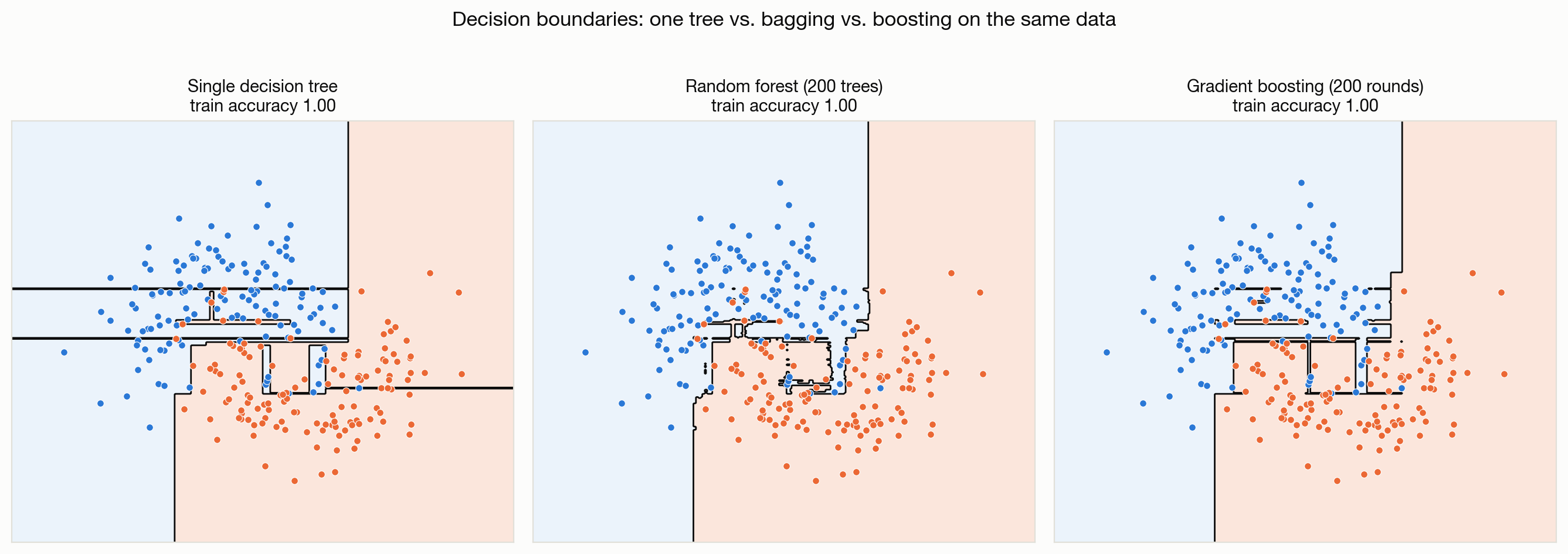
All three models reach perfect or near-perfect training accuracy, which is exactly the trap: training accuracy alone cannot distinguish the single tree’s memorized, jagged boundary from the ensembles’ smoother, more plausible ones. Only held-out evaluation reveals the difference in generalization.
4.2 Main methods
Decision trees (CART). The base unit. Interpretable — you can read off the exact sequence of decisions leading to any prediction — and useful on their own as a fast baseline or when explainability is a hard requirement, but rarely competitive on accuracy alone once other options are available. Regularized via max depth, minimum samples per leaf, minimum impurity decrease, or post-hoc cost-complexity pruning.
Random forests. Bagging plus random feature subsets, as derived above. Robust, hard to badly misconfigure (few sensitive hyperparameters, and performance is fairly flat across a wide range of tree counts and depths), naturally parallel to train (every tree is independent), and provides out-of-bag error estimates for free (each tree can be validated on the ~37% of bootstrap samples it never saw). Weaker than boosting on raw predictive accuracy in most benchmarks, but a very safe default.
Gradient boosted trees. Sequential residual-fitting as derived above. Typically the strongest out-of-the-box performer on tabular data, but has more hyperparameters that actually matter (learning rate, number of rounds, tree depth, subsampling fraction, regularization terms) and needs early stopping on a validation set to avoid overfitting, since — unlike a random forest — adding more rounds can and eventually will hurt generalization.
XGBoost, LightGBM, CatBoost. Three production-grade gradient boosting implementations that differ mainly in engineering tradeoffs rather than the core algorithm. XGBoost added a formal regularization term to the tree-split objective (a second-order Taylor approximation of the loss, penalizing leaf weights and leaf count) and highly optimized, cache-aware split-finding. LightGBM grows trees leaf-wise (always splitting whichever leaf most reduces loss) rather than level-wise, which is faster and often more accurate for a given leaf budget but more prone to overfitting on small data, and uses histogram-based binning of continuous features for speed. CatBoost’s distinguishing feature is native, statistically careful handling of categorical features (via ordered target statistics that avoid leaking label information) without manual one-hot or target encoding, plus symmetric (“oblivious”) trees that are faster to evaluate at inference time. In practice all three are strong; the choice is usually about categorical feature handling, training speed at your data scale, and inference latency constraints rather than a large gap in achievable accuracy.
ExtraTrees and other bagging variants. Extremely Randomized Trees push the randomization in random forests one step further by also randomizing the split threshold for each candidate feature (rather than exhaustively searching for the best threshold), trading a little bias for faster training and sometimes even lower variance. Useful when random forest training time is a bottleneck.
4.3 When to use it / what can go wrong
Tree ensembles are usually the right first model to reach for on structured, tabular data — mixed numeric and categorical features, moderate size (thousands to low millions of rows), where feature interactions matter and you don’t already have strong domain knowledge about the functional form. They need essentially no feature scaling (splits are threshold comparisons, invariant to monotonic transformations), handle missing values natively in most modern implementations, and give you feature importance and single-tree visualizations as debugging tools for free.
Poor fit for raw unstructured input. Trees split on individual feature thresholds, which is a poor match for raw pixels, audio waveforms, or token sequences, where the meaningful structure is in spatial or sequential relationships between many correlated dimensions rather than a threshold on any one of them. This is squarely where deep learning’s inductive biases (convolution, attention) earn their keep instead. Tree ensembles remain strong, however, once such data has been reduced to engineered or learned features — a tabular model stacked on top of embeddings is a common and effective pattern.
Calibration is not automatic. Gradient boosted trees in particular tend to produce poorly calibrated probability outputs, especially with the log-loss objective pushed hard by many rounds — predicted probabilities cluster near 0 and 1 more than the true event frequencies warrant. If a downstream system consumes the score as a genuine probability, check a reliability diagram and apply post-hoc calibration (Platt scaling or isotonic regression) rather than assuming boosted-tree output is well-calibrated by construction.
Serving cost at scale. A production gradient-boosted model can easily contain thousands of trees; evaluating all of them for every prediction adds real latency and memory cost compared to a linear model or a compact neural network, which matters for high-QPS, low-latency serving paths or constrained on-device deployment. This is one reason tree ensembles are common for offline scoring or as a candidate-generation/reranking stage but less common as the final hop in a sub-10ms latency budget.
Poor extrapolation. Because trees predict a constant value within each leaf’s region, and leaf regions are bounded by the range of the training data, a tree ensemble cannot extrapolate beyond the feature ranges it was trained on — a linear model will at least produce a directionally sensible (if possibly wrong) prediction outside its training range, while a tree ensemble simply predicts the value of whatever leaf boundary it saturates against. This matters for any feature that drifts over time (prices, counts, dates) where production inputs will eventually exceed the training distribution’s range.
4.4 How this connects
- Supervised Learning is the general ERM framework this chapter specializes: trees replace the linear or logistic functional form with a recursively partitioned, non-parametric one, but the underlying bias-variance tension, loss function choice, and overfitting risk are identical.
- Deep Learning Foundations is the natural point of comparison for any new tabular problem — the “GBDT vs. neural net” decision usually comes down to data size, whether features are structured or raw, interpretability requirements, and serving latency, and GBDTs remain the stronger default on small-to-medium tabular data even in the deep learning era.
- Information Retrieval, Ranking, and Recommenders relies heavily on boosted trees: LambdaMART and related learning-to-rank objectives are gradient boosting with a pairwise or listwise loss in place of pointwise squared error or log-loss, built on exactly the machinery derived above.
- Evaluation and Benchmarking covers the calibration diagnostics (reliability diagrams, Brier score decomposition) needed to catch the miscalibration failure mode flagged above before it reaches production.
- ML Systems and MLOps is where the serving-cost tradeoff between a thousand-tree ensemble and a compact model actually gets resolved, through techniques like tree distillation, quantization, or restricting ensemble size for latency-critical serving paths.