9 Deep Learning Foundations
Deep learning is, at its mathematical core, a strikingly simple idea applied with enormous discipline: compose many simple differentiable functions into one large function, and use the fact that composition is differentiable to adjust every internal parameter by gradient descent until the whole thing does something useful. Each individual layer — a linear transform followed by a nonlinearity — is not very expressive on its own. Stacked into dozens or hundreds of layers, with enough parameters and enough data, the composed function can approximate extraordinarily rich relationships: pixels to object categories, audio waveforms to text, protein sequences to 3D structure, token sequences to fluent continuations. The word “deep” refers literally to this stacking; the power comes not from any single layer being clever, but from depth letting the network build increasingly abstract representations on top of simpler ones, and from that whole stack being trainable end-to-end by one algorithm.
That last point is the real story of this chapter. Backpropagation and gradient-based optimization are not implementation detail — they are the reason deep learning works as a general-purpose method at all. Before efficient, reliable gradient-based training of deep composed functions, getting a many-layer model to learn anything useful was a research problem in itself. Understanding how gradients flow backward through a deep network, what makes that flow break down, and what the fixes (initialization, normalization, better optimizers, architectural changes) actually correct for is the difference between using deep learning as a black box and actually being able to debug it when it doesn’t work.
9.1 How it works
Backpropagation: the chain rule at scale
A deep network is a composition of functions, layer by layer: \(\hat y = f_L(f_{L-1}(\cdots f_1(x) \cdots))\), where each \(f_\ell\) has parameters \(\theta_\ell\) (weights and biases) and typically ends with a nonlinear activation. Training minimizes a loss \(\mathcal{L}(\hat y, y)\) over these parameters using gradient descent, which needs \(\partial \mathcal{L} / \partial \theta_\ell\) for every layer. Backpropagation computes all of these efficiently using the chain rule, applied backward through the computation graph: starting from \(\partial \mathcal{L} / \partial \hat y\) at the output, each layer receives the gradient of the loss with respect to its output, computes the gradient with respect to its own parameters (to update them) and the gradient with respect to its input (to hand backward to the previous layer), one layer at a time:
\[ \frac{\partial \mathcal{L}}{\partial \theta_\ell} = \frac{\partial \mathcal{L}}{\partial f_L} \cdot \frac{\partial f_L}{\partial f_{L-1}} \cdots \frac{\partial f_{\ell+1}}{\partial f_\ell} \cdot \frac{\partial f_\ell}{\partial \theta_\ell}. \]
The key efficiency insight is that this is computed once, layer by layer, reusing the downstream gradient at every step, rather than recomputing the full chain rule product separately for every parameter — which is what makes training networks with millions or billions of parameters computationally feasible at all: the cost of one backward pass is a small constant multiple of one forward pass, independent of how many parameters you’re differentiating with respect to.
Why deep networks are hard to train, and what fixes that
The chain-rule product above is also the source of deep learning’s central practical failure mode. Each factor \(\partial f_{\ell+1}/\partial f_\ell\) is typically less than 1 in magnitude for saturating activations (sigmoid, tanh) or can be greater or less than 1 depending on the weight scale for others. Multiply many such factors together across dozens of layers, and the product can shrink toward zero (vanishing gradients, early layers essentially stop learning because no signal reaches them) or blow up toward infinity (exploding gradients, updates become unstable). This isn’t a minor numerical nuisance — it’s the reason naively stacking many layers used to make networks harder to train, not easier, and it explains why several of deep learning’s core techniques all exist to solve exactly this one problem from different angles:
- Activation functions. ReLU (\(\max(0, x)\)) and its variants replaced sigmoid/tanh as the default hidden-layer activation largely because their gradient is either exactly 1 or exactly 0, not a fraction less than 1 — this removes one major source of vanishing gradients (at the cost of “dead” units whose gradient is permanently 0 if they always output negative pre-activations, which motivated variants like Leaky ReLU and GELU).
- Initialization. Schemes like Xavier/Glorot and He initialization set the initial weight variance as a function of layer width specifically so that activations and gradients start out with roughly constant variance as they pass through layers, rather than shrinking or growing multiplicatively from the first forward/backward pass.
- Normalization. Batch normalization and layer normalization re-center and re-scale activations partway through the network (per mini-batch across the batch dimension for BatchNorm; per example across the feature dimension for LayerNorm, which is what transformers use since it doesn’t depend on batch statistics) so that the distribution of values flowing into each layer stays stable during training, which both stabilizes gradient flow and, empirically, lets you use larger learning rates.
- Architectural shortcuts. Residual connections (as in ResNets and every modern transformer) add the input of a block directly to its output, \(y = x + f(x)\), so that the gradient has a direct path backward through the “+x” term with derivative exactly 1, regardless of how small \(\partial f/\partial x\) is. This is arguably the single architectural change that made networks with hundreds of layers trainable at all.
Gradient descent variants and why momentum and adaptivity help
Plain (stochastic) gradient descent updates parameters by \(\theta \leftarrow \theta - \eta \nabla_\theta \mathcal{L}\). This is simple but can be painfully slow on loss surfaces with very different curvature in different directions — a narrow curved valley, for instance, where the gradient points mostly across the valley (steep direction) rather than along it (the direction that actually leads toward the minimum). Momentum accumulates a running average of past gradients, \(v \leftarrow \beta v + \nabla_\theta \mathcal{L}\), \(\theta \leftarrow \theta - \eta v\), which reinforces consistent gradient directions across steps and damps oscillation in directions where the gradient keeps flipping sign — but because it keeps “velocity” from previous steps, it can overshoot a minimum and oscillate before settling. Adam goes further, maintaining per-parameter running estimates of both the gradient’s mean (first moment, like momentum) and its squared magnitude (second moment), then normalizing the update by the square root of that second moment — effectively giving each parameter its own adaptive step size, taking larger steps for parameters with consistently small gradients and smaller steps for parameters with large or noisy gradients. This adaptivity is why Adam is a robust default for deep learning: it needs less manual learning-rate tuning and handles the very differently-scaled gradients that different layers of a deep network naturally produce.
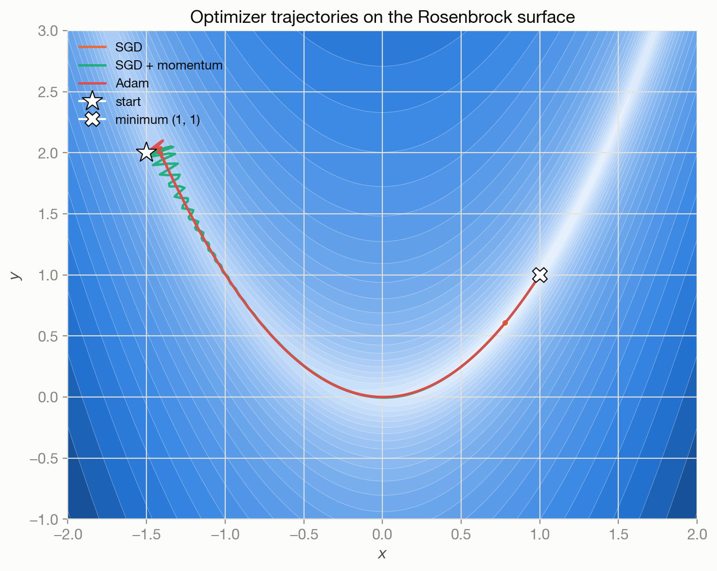
Figure 9.1 visualizes exactly this difference on the Rosenbrock function, a classic non-convex test surface with a long, narrow, curved valley — a deliberately hard case for optimization because the gradient direction and the direction toward the minimum are often nearly perpendicular. Starting all three optimizers from the same point makes the qualitative differences visible directly as paths: plain SGD with a small, stable learning rate creeps slowly down the valley wall and only makes modest progress along the valley floor in a fixed step budget; SGD with momentum picks up “velocity” and visibly oscillates back and forth across the narrow valley before it manages to align with the valley’s direction; Adam’s per-parameter adaptive scaling lets it descend the steep wall and then accelerate along the shallow valley floor efficiently, reaching much closer to the true minimum at \((1, 1)\) in the same number of steps.
Attention, briefly derived
The other essential mechanism worth deriving is attention, since it underlies transformers and most of modern sequence and multimodal modeling. For a sequence of token representations, attention lets each token build a new representation as a weighted combination of every token’s value vector, with weights determined by how relevant each token is to the one being updated. Concretely, each token produces a query vector \(q\) (what it’s looking for), a key vector \(k\) (what it offers to be matched against), and a value vector \(v\) (the information it contributes if selected). The attention weights come from query-key similarity, scaled and normalized:
\[ \text{Attention}(Q, K, V) = \text{softmax}\!\left(\frac{QK^\top}{\sqrt{d_k}}\right) V, \]
where \(Q, K, V\) stack the queries, keys, and values for every token, and the \(\sqrt{d_k}\) scaling keeps the dot products (and hence the softmax) from saturating as the key dimension \(d_k\) grows. Unlike a recurrent network, which must pass information through a fixed-size hidden state one step at a time, self-attention lets any token attend directly to any other token in a single layer, regardless of distance between them — this is the mechanism that gives transformers their strength on long-range dependencies and their parallelizability across the sequence dimension during training (every token’s attention output can be computed simultaneously, unlike a recurrence, which is inherently sequential). The cost is quadratic complexity in sequence length, since every token attends to every other token — a central engineering constraint discussed further in Sequence, Time-Series, and State Models.
9.2 Main methods
Architecture families
- MLPs (multi-layer perceptrons) are the generic case: fully-connected layers with no assumption about input structure. They’re the right default for tabular or unstructured feature vectors, and the building block inside every other architecture (the feed-forward sublayer in a transformer block is an MLP).
- CNNs (convolutional networks) encode a strong prior for spatial structure: a small filter is applied at every spatial location with shared weights, which builds in translation invariance and drastically reduces parameter count compared to a fully-connected layer over the same input, at the cost of needing that spatial-locality assumption to be roughly true.
- RNNs and LSTMs process sequences by maintaining a hidden state updated one step at a time, giving them a natural fit for sequential data and, unlike a fixed-window model, in principle unbounded context — covered in depth alongside the vanishing-gradient problem they specifically struggle with in Sequence, Time-Series, and State Models.
- Transformers replace recurrence with the self-attention mechanism above, trading recurrence’s sequential processing for parallelizable, any-to-any token interaction, and currently dominate large-scale language, vision, and multimodal modeling.
- Graph neural networks generalize the same “aggregate information from a structured neighborhood” idea to arbitrary graphs rather than grids or sequences — covered in Graph Neural Networks and Structured Data.
Regularization
A model with enough parameters can memorize its training data outright, achieving low training loss while generalizing poorly — the classic overfitting failure covered generally in Supervised Learning. Deep learning has its own toolkit for fighting this: dropout randomly zeroes a fraction of activations during training, which prevents units from co-adapting to compensate for each other’s specific quirks and acts like training an implicit ensemble of subnetworks; weight decay penalizes large weights directly in the loss, encouraging simpler functions (and is mathematically a Gaussian prior on the weights in a Bayesian reading — the same regularization-as-prior connection covered in Probabilistic Modeling); early stopping halts training once validation performance stops improving, using the optimization trajectory itself as an implicit regularizer instead of a loss penalty.
Transfer learning and scale
Rather than training from scratch, transfer learning starts from a model already trained on a large, related dataset and adapts it — either by fine-tuning all its weights on a smaller task-specific dataset, or by freezing most of the network and only training a new final layer. This works because the representations learned earlier in the network (edges and textures in vision, syntax and word relationships in language) tend to be broadly reusable, while the later layers specialize to the specific task; it turns a small-data problem into a small-adaptation-of-a-large-model problem. At the far end of this idea are scaling laws: empirical regularities showing that model loss decreases smoothly and predictably as a power law in model size, dataset size, and compute, provided the three are scaled together in roughly the right ratio. This observation is the intellectual basis of the foundation-model paradigm covered in Generative AI and Foundation Models: train one very large model on a very large, broad dataset once, then adapt or prompt it for many downstream tasks, rather than training many small task-specific models from scratch.
9.3 When to use it / what can go wrong
Data leakage — information from outside the legitimate training data influencing the model, whether through a preprocessing step fit on the full dataset before splitting, a duplicated example spanning train and test, or a feature that encodes the label — inflates offline metrics and is one of the most common reasons a model that looked excellent in evaluation underperforms badly once deployed. This is a general ML risk, but deep learning’s appetite for large, often loosely curated datasets makes it especially easy to introduce without noticing.
Shortcut learning happens when a network finds a spurious correlation that predicts the label on the training distribution without capturing the actual underlying task — a classic example is a model that learns to detect a watermark or image artifact correlated with one class rather than the class itself. It produces strong benchmark numbers and brittle real-world behavior, and it’s hard to catch without deliberately testing on out-of-distribution or adversarially constructed examples.
Poor calibration. A deep network’s softmax output is not automatically a trustworthy probability — large networks are frequently overconfident, assigning high probability to wrong predictions, especially outside the training distribution. Where downstream decisions depend on confidence (risk-sensitive ranking, human handoff thresholds, active learning), raw softmax scores should be treated with suspicion and calibrated, or paired with a genuinely distribution-free method like the ones in Conformal Prediction.
Distribution shift between training and deployment — different user population, different sensor characteristics, drift over time — degrades a deep model the same way it degrades any statistical model, but deep models’ opacity makes the degradation harder to diagnose: there’s no small set of coefficients to inspect for what changed.
Expensive inference and hard-to-debug failures. Depth and scale that buy accuracy also buy latency, memory, and serving cost, which is often the binding constraint on what can actually ship — see ML Systems and MLOps. And because a deep network’s decision is distributed across millions or billions of parameters with no individually interpretable meaning, root-causing a specific bad prediction is fundamentally harder than debugging a linear model or a small decision tree — this tradeoff between raw capability and interpretability recurs constantly and is worth weighing explicitly rather than defaulting to the largest model available.
9.4 How this connects
- Representation Learning supplies the motivating goal — learned, task-useful internal representations — that the architectures and training techniques in this chapter exist to produce; the encoder/decoder networks in an autoencoder or VAE are built from exactly the layers and trained with exactly the optimizers covered here.
- Sequence, Time-Series, and State Models goes deep on the RNN/LSTM/transformer family sketched above, including why RNNs specifically suffer from vanishing gradients across time steps and how attention’s quadratic cost shapes real serving constraints.
- Graph Neural Networks and Structured Data extends the same layered, differentiable, gradient-trained paradigm to graph-structured data, replacing convolution’s grid neighborhood or attention’s full sequence with message passing over graph edges.
- Probabilistic Modeling underlies the loss functions used to train these networks (cross-entropy is maximum likelihood under a categorical model; weight decay is a Gaussian prior) and the calibration concerns raised above.
- ML Systems and MLOps is where the practical costs mentioned above — inference latency, training compute, model size — turn into the actual constraints that decide which architecture and which scale of model can ship in a real system.