14 Generative AI and Foundation Models
A discriminative model answers “given this input, what’s the label?” A generative model answers a harder question: “what does the data itself look like, and can I produce more of it?” Learning \(p(x)\) — or \(p(x \mid c)\) for some conditioning signal \(c\) like a text prompt — is a strictly harder estimation problem than learning a decision boundary, because a generative model has to get the whole joint structure of the data right, not just the parts that happen to separate classes. The payoff is that once you have a good model of \(p(x)\), you can sample from it: write new text, draw a new image, propose a new molecule, synthesize a new voice. Everything in this chapter is a different answer to the same question — how do you parameterize and train a model that can sample realistic data — and a foundation model is simply one of these generative (or self-supervised predictive) models trained at enormous scale on broad data, then adapted to many downstream tasks rather than built for one.
The field converged on a small number of families because each one makes a different, deliberate trade among three things every generative model wants: exact likelihoods (so you can train by maximum likelihood and know exactly how much probability mass you’re assigning to each point), high sample quality (so what you generate actually looks/reads right), and fast sampling (so generation isn’t prohibitively slow). No family gets all three for free — autoregressive models get exact likelihoods and great quality but sample slowly, one token at a time; GANs sample in one shot but abandon likelihoods entirely; diffusion models get excellent quality and a tractable (if approximate) likelihood bound at the cost of many sampling steps. Once you see the trade-off, the zoo of architectures stops looking arbitrary.
14.1 How it works
The likelihood-based view
Most of what follows is united by trying to maximize the log-likelihood of observed data under a model \(p_\theta\):
\[ \theta^\star = \arg\max_\theta \; \mathbb{E}_{x \sim p_{\text{data}}} \left[ \log p_\theta(x) \right] \]
The families differ in how they make \(p_\theta(x)\) tractable to evaluate and optimize.
Autoregressive models use the chain rule of probability to factor a joint distribution over a sequence \(x = (x_1, \dots, x_n)\) into a product of conditionals:
\[ p_\theta(x) = \prod_{i=1}^{n} p_\theta(x_i \mid x_1, \dots, x_{i-1}) \]
This factorization is exact — no approximation, no independence assumption — so the log-likelihood is exactly computable and directly optimizable by gradient descent. This is precisely what a large language model does: each conditional \(p_\theta(x_i \mid x_{<i})\) is “predict the next token given everything so far,” parameterized by a transformer’s output softmax. The same idea underlies autoregressive image models (PixelCNN-style, and patch-autoregressive vision-language models) and autoregressive audio codecs. The cost is serial sampling: producing \(x_n\) requires having already produced \(x_1, \dots, x_{n-1}\), so generation time scales with sequence length and can’t trivially parallelize.
Diffusion models take a different route to a tractable likelihood bound. Instead of factoring \(p(x)\) directly, they define a fixed, simple forward process that gradually destroys structure in the data by adding noise over \(T\) steps, and then train a neural network to learn the reverse process that removes noise one step at a time. The forward process is a Markov chain with Gaussian transitions:
\[ q(x_t \mid x_{t-1}) = \mathcal{N}\!\left(x_t;\ \sqrt{1-\beta_t}\, x_{t-1},\ \beta_t I\right) \]
for a variance schedule \(\beta_1, \dots, \beta_T\). Because Gaussians compose nicely, this has a closed form for jumping straight from the clean data \(x_0\) to any noise level \(t\) without simulating the intermediate steps:
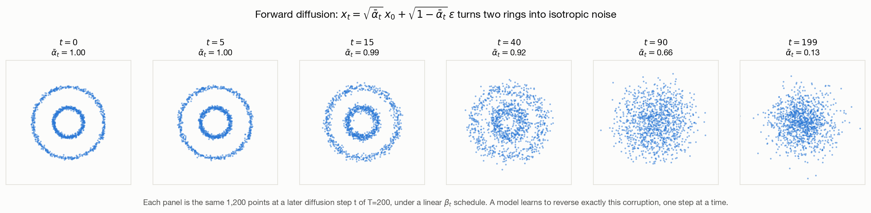
\[ x_t = \sqrt{\bar\alpha_t}\, x_0 + \sqrt{1-\bar\alpha_t}\, \varepsilon, \qquad \varepsilon \sim \mathcal{N}(0, I), \qquad \bar\alpha_t = \prod_{s=1}^{t}(1-\beta_s) \]
Figure 14.1 runs exactly this equation on a toy 2D distribution (points shaped like two concentric rings) and shows the point cloud at increasing \(t\): the rings blur, then dissolve entirely into isotropic Gaussian noise by \(t=T\). Nothing here is learned yet — this is purely the fixed corruption process. The generative model’s whole job is to learn to invert it: given a noisy \(x_t\), predict either the noise \(\varepsilon\) that was added or the clean \(x_0\) underneath it. Training reduces to a simple regression loss — predict the noise, minimize squared error — which is why diffusion training is remarkably stable compared to adversarial training. Why does denoising suffice to learn the whole data distribution? Because the noise-prediction target at each step is (up to a reweighting) a Monte Carlo estimate of the score function \(\nabla_x \log p_t(x)\) of the noised data distribution at that noise level, and having the score at every noise level lets you walk from pure noise back to the data manifold one small, locally-accurate step at a time — this is the score-based / stochastic-differential-equation view of diffusion, and it’s why diffusion models are sometimes described as learning to “denoise their way downhill” toward high-density regions of the data.
Variational autoencoders (VAEs) take a latent-variable approach: assume each observation \(x\) is generated from some unobserved code \(z\) via \(p(z) \to p_\theta(x \mid z)\), with \(p(z)\) a simple prior (usually \(\mathcal{N}(0, I)\)). The marginal likelihood \(p_\theta(x) = \int p_\theta(x \mid z)\, p(z)\, dz\) is intractable, so a VAE trains an encoder \(q_\phi(z \mid x)\) to approximate the true posterior and optimizes the evidence lower bound (ELBO):
\[ \log p_\theta(x) \geq \mathbb{E}_{q_\phi(z\mid x)}\!\left[\log p_\theta(x \mid z)\right] - D_{\mathrm{KL}}\!\left(q_\phi(z\mid x) \,\|\, p(z)\right) \]
the reconstruction term pulling samples toward faithfully decoding \(z\) back into \(x\), and the KL term regularizing the learned posterior toward the prior so that sampling \(z \sim p(z)\) at generation time actually lands somewhere the decoder has seen. This connects VAEs directly to the latent-variable models covered in Graphical Models and Latent Variables — a VAE is exactly that kind of model, just with the E-step replaced by an amortized neural network and exact inference replaced by a variational bound.
GANs sidestep likelihoods altogether. A generator \(G\) maps noise \(z \sim p(z)\) to samples \(G(z)\), and a discriminator \(D\) is trained to distinguish real data from \(G\)’s output; \(G\) is trained to fool \(D\). The minimax objective
\[ \min_G \max_D \; \mathbb{E}_{x \sim p_{\text{data}}}[\log D(x)] + \mathbb{E}_{z \sim p(z)}[\log(1 - D(G(z)))] \]
has no explicit likelihood term at all — quality is defined implicitly by whatever the discriminator can’t detect. This buys single-shot sampling (no iterative denoising, no autoregressive unrolling) at the cost of notoriously unstable training: \(G\) and \(D\) are chasing a moving target in each other, and there’s no loss curve that reliably tells you “training is going well” the way there is for a regression loss.
Normalizing flows keep exact likelihoods by construction: they learn an invertible transformation \(f_\theta\) from a simple base distribution (e.g. Gaussian) to the data distribution, and the change-of-variables formula gives the likelihood exactly:
\[ \log p_\theta(x) = \log p_{\text{base}}(f_\theta^{-1}(x)) + \log \left|\det \frac{\partial f_\theta^{-1}(x)}{\partial x}\right| \]
The catch is architectural: \(f_\theta\) must be invertible with a tractable Jacobian determinant, which rules out most of the free-form expressiveness available to the other families, so flows tend to need more layers/capacity to match the sample quality of diffusion or autoregressive models on complex data like natural images.
Tokenization and next-token prediction
Before any of this can run on text, text has to become numbers. Modern LLMs use subword tokenization — byte-pair encoding (BPE) or a close variant — which builds a vocabulary by starting from individual bytes or characters and iteratively merging the most frequent adjacent pair until reaching a target vocabulary size (commonly 32k–200k tokens). This is a compromise: word-level tokenization has an unbounded vocabulary and can’t represent unseen words; character-level tokenization has a tiny vocabulary but very long sequences (worse compute cost, since attention cost grows with sequence length). Subword tokenization gets common words as single tokens and rare words as a few subword pieces, so vocabulary stays fixed-size and sequences stay reasonably short. Given a tokenizer, a decoder-only transformer is trained with exactly the autoregressive factorization above: given tokens \(x_{<i}\), predict a distribution over the next token, and minimize cross-entropy against the actual next token in the training corpus. This single, simple objective — no labels beyond “what comes next” — is what makes pretraining scalable: any text on the internet is training data.
From pretraining to a usable assistant
A raw pretrained LLM is a very good next-token predictor over its training distribution, which is not the same thing as a helpful assistant — it will happily continue a question with more questions, because that’s a plausible continuation of internet text. Getting from there to something like a modern chat assistant is a further sequence of training stages:
- Instruction tuning (supervised fine-tuning, SFT): fine-tune on (instruction, desired response) pairs, usually written or curated by humans, so the model’s default behavior shifts from “continue this text” to “follow this request.”
- Preference tuning: collect pairs of model outputs with human (or AI) preference judgments about which is better, and optimize the model to prefer the better one. RLHF does this via a learned reward model plus policy-gradient RL (typically PPO) — connecting straight to Reinforcement Learning and Bandits, since the LLM is literally the policy and each generated response is a trajectory scored by a scalar reward. Direct Preference Optimization (DPO) and its relatives reformulate the same preference signal as a closed-form classification loss on pairs, without training a separate reward model or running RL rollouts — cheaper and more stable, at the cost of being less naturally suited to reward signals that aren’t simple pairwise preferences (e.g. rewarding correctness on a verifiable task, where RL with a programmatic reward — as in RLVR / RL-from-verifiable-rewards used for math and code reasoning models — still has a clear advantage).
- RAG (retrieval-augmented generation): rather than relying purely on facts baked into weights during pretraining, retrieve relevant documents at inference time (via the embeddings and search machinery in Information Retrieval, Ranking, and Recommenders) and condition generation on them. This trades a fixed, stale, opaque parametric memory for a memory that’s current, inspectable, and updatable without retraining — at the cost of being only as good as the retriever, and introducing a new failure mode where the model ignores or misinterprets the retrieved context.
Multimodal models
Text, images, audio, and video increasingly live in shared model families rather than separate pipelines. The common recipe is to make every modality speak the same representational language: a vision encoder (often a ViT-style patch encoder, sometimes contrastively pretrained like CLIP) maps an image to a sequence of embeddings that get projected into the same space the language model’s token embeddings live in, so “image tokens” and text tokens can be attended over jointly by one transformer. Contrastive pretraining — pulling matching (image, caption) pairs together in embedding space and pushing mismatched pairs apart — gives a modality-agnostic embedding space useful for retrieval and zero-shot classification even before any generative training happens. Cross-attention is the other common glue: a text decoder that attends into a separately-encoded image or audio stream, keeping the modality-specific encoder architecturally separate while letting information flow at generation time. Diffusion has become the dominant generative mechanism for images/video/audio specifically because sample quality and mode coverage (not collapsing onto a few typical outputs, which plagued GANs) matter enormously for perceptual media, and diffusion’s training stability makes it practical to scale.
14.2 Main methods
The table below is really the same summary as the trade-off framing above, now organized by what you’d actually reach for:
- Decoder-only transformer LLMs (GPT-, Llama-, Claude-, Gemini-style): the default for text and code generation. Exact likelihoods, excellent quality, but inherently serial sampling — this is why LLM inference latency scales with output length and why techniques like speculative decoding (drafting several tokens with a cheap model, verifying them in parallel with the real model) exist purely to claw back throughput.
- Diffusion models (Stable Diffusion / DALL-E / Imagen-style for images, and increasingly for video and audio): the default for continuous, perceptual media where sample diversity and quality both matter. Sampling requires many denoising steps, though distillation techniques (consistency models, few-step samplers) have pushed this down from ~1000 steps to single digits in some production systems.
- VAEs: rarely the end-to-end generator of choice for top-quality samples anymore (they tend to produce blurrier outputs than diffusion or GANs, a direct consequence of the reconstruction term in the ELBO being an average over the whole posterior), but the encoder/decoder architecture is ubiquitous as a component — e.g. the latent-space compression stage in latent diffusion models runs an image through a VAE encoder before diffusion operates in the smaller latent space, and back through the decoder to produce pixels.
- GANs: still relevant for applications needing fast, single-shot, high-fidelity sampling at fixed resolution (some face/style-transfer and real-time applications), but have been largely displaced from general-purpose image generation by diffusion’s better mode coverage and training stability.
- Normalizing flows: rarely the top choice for sample quality on complex high-dimensional data, but valuable whenever you specifically need exact, tractable density evaluation — e.g. as a component in some variance-reduction or importance-sampling schemes, or in scientific applications wanting a genuine likelihood, not just samples.
14.3 When to use it / what can go wrong
Choosing a family is mostly answering: do you need exact likelihoods (pick autoregressive or flows), do you need best-in-class perceptual quality and can tolerate multi-step sampling (pick diffusion), do you need one-shot fast sampling and can tolerate training instability (consider GANs)? For text specifically, autoregressive transformers are close to the only practical choice today, since language’s discrete, sequential structure suits the chain-rule factorization far better than it suits diffusion (text diffusion models exist and are an active research area, mainly attractive for parallel/non-autoregressive decoding speed, but haven’t displaced autoregressive LLMs in production as of 2026).
Evaluation is genuinely hard, and harder than for discriminative models, because a generative model rarely has one correct output — many different continuations, images, or answers can all be “right.” Surface metrics like perplexity measure how well a model predicts held-out text under its own objective, but a lower perplexity doesn’t guarantee more helpful, more factual, or more preferred outputs — this is exactly the kind of offline-metric/product-outcome divergence covered in depth in Evaluation and Benchmarking. For instruction-tuned models specifically, you care about a different bundle of properties than raw likelihood: factuality (are claims true), groundedness (are claims actually supported by retrieved/provided context, distinct from being true in general — a model can state something true but not have gotten it from the context it was given), helpfulness, safety, and diversity (a model collapsed onto a few stock phrasings has a problem even if each individual output looks fine). None of these are single numbers computable from logits alone, which is why human preference judgments and LLM-as-judge evaluation became central rather than incidental to how generative models get assessed.
Concrete failure modes worth having a name for: mode collapse (a GAN’s generator finds a handful of outputs that reliably fool the current discriminator and stops producing anything else — diversity collapses even as individual samples look fine); posterior collapse in VAEs (the decoder learns to ignore \(z\) entirely and the KL term drives \(q_\phi(z\mid x)\) to match the prior with no information about \(x\), especially with a powerful autoregressive decoder that doesn’t need the latent to reconstruct well); exposure bias in autoregressive models (trained on ground-truth prefixes but sampled from its own, imperfect prefixes at inference time, so small errors early in generation can compound); and, for RAG, retrieval failure silently becoming generation failure — if the retriever returns irrelevant documents, a well-trained model will often still confidently synthesize an answer from them rather than flagging that nothing useful was found.
14.4 How this connects
- Graphical Models and Latent Variables — a VAE is a latent-variable model with an amortized, neural variational posterior; the ELBO here is the same evidence lower bound derived there.
- Sampling and Approximate Inference — diffusion sampling is literally an iterative stochastic sampling procedure, and the forward/reverse process view connects directly to score-based sampling and Langevin dynamics.
- Sequence, Time-Series, and State Models — autoregressive LLMs are sequence models; the transformer architecture and attention mechanism live there.
- AI Agents, Tool Use, and Multi-Agent Systems — agents are built on top of exactly the instruction-tuned, tool-calling foundation models described here; tool calling is a structured-generation extension of next-token prediction.
- Evaluation and Benchmarking — generative model evaluation (factuality, groundedness, human preference, LLM-as-judge) is developed in full there rather than repeated per-chapter.
- Reinforcement Learning and Bandits — RLHF treats the LLM as a policy and human/reward-model preferences as reward, making preference tuning a direct application of policy-gradient RL.