16 Evaluation and Benchmarking
Every other chapter in this book asks “how do you build X.” This one asks a question that cuts across all of them: how do you know whether what you built actually works? That sounds like it should be the easy part — compute a metric, check if it went up — but “how do you evaluate this” turns out to be its own deep methodological problem, with its own failure modes, that apply just as much to a gradient-boosted tree as to a frontier LLM. A number that looks like rigor (a benchmark score, a leaderboard rank, an accuracy to three decimal places) can be nearly meaningless if it was measured wrong, measured on the wrong thing, or measured on data the model has effectively already seen. This chapter is about the gap between a metric and the truth it’s supposed to stand in for, and the toolkit for closing that gap: held-out evaluation, calibration, human and automated judgment, and the statistical discipline to know when a difference is real.
16.1 How it works
Held-out metrics and why they diverge from product outcomes
The basic discipline of machine learning evaluation — compute a metric on data the model didn’t train on — exists to answer one narrow question: does this model generalize, or did it just memorize? A held-out test set answers that question honestly only if it’s drawn from the same distribution the model will actually face and is never used to make modeling decisions (that’s what a separate validation set is for). Get that right and you still haven’t answered the question anyone actually cares about, which is usually not “what is this model’s held-out log-loss” but “does using this model make the product better” — more revenue, more satisfied users, more tasks completed correctly. These two things diverge for concrete, recurring reasons:
- Metric-proxy mismatch: the offline metric is a proxy for what you actually want, and proxies leak. A recommender optimized for click-through rate can learn to recommend clickbait that users regret clicking, so offline CTR improves while satisfaction (the thing you actually wanted) gets worse. A next-token-prediction loss can improve while the model gets no more helpful at the tasks users actually bring it. This is the same phenomenon Goodhart’s law describes — once a proxy becomes the target, optimization pressure finds ways to move the proxy that don’t move the underlying goal.
- Distribution shift between offline and online: a held-out set is a fixed snapshot; the real traffic distribution drifts (new users, new query types, seasonal effects, adversarial or novel inputs), so a metric computed once, offline, degrades in relevance over time even without the model changing at all. See ML Systems and MLOps for how this shows up as production drift monitoring.
- Aggregate metrics hide subgroup and tail behavior: a metric averaged across the whole test set can look great while a model fails badly on a minority segment, a rare-but-important query type, or exactly the hardest cases that matter most to get right. Because the average is dominated by the common case, a subgroup that’s 2% of the traffic can fail completely and move the headline number by a rounding error.
None of this means offline metrics are useless — they’re cheap, fast, and reproducible in a way online tests aren’t, and they’re indispensable for day-to-day model iteration. It means an offline metric is necessary but not sufficient, and the final arbiter of whether a change actually helped has to be closer to the real outcome, which is what the online evaluation section below is about.
Calibration and reliability diagrams
A model that outputs a probability makes an additional, checkable claim beyond “which class is most likely”: it claims that among all the times it says “70% confident,” it should be right about 70% of the time. That property is calibration, and it’s a genuinely different axis from accuracy — a model can be highly accurate and badly calibrated (right most of the time, but overconfident when it’s wrong), or poorly discriminative but well calibrated (correctly humble, but not very useful for ranking cases by risk). Calibration matters wherever a downstream decision consumes the probability itself, not just the top prediction — thresholding for review queues, expected-value calculations, risk stratification in medical or lending contexts, or an LLM’s stated confidence being used to decide whether to defer to a human.
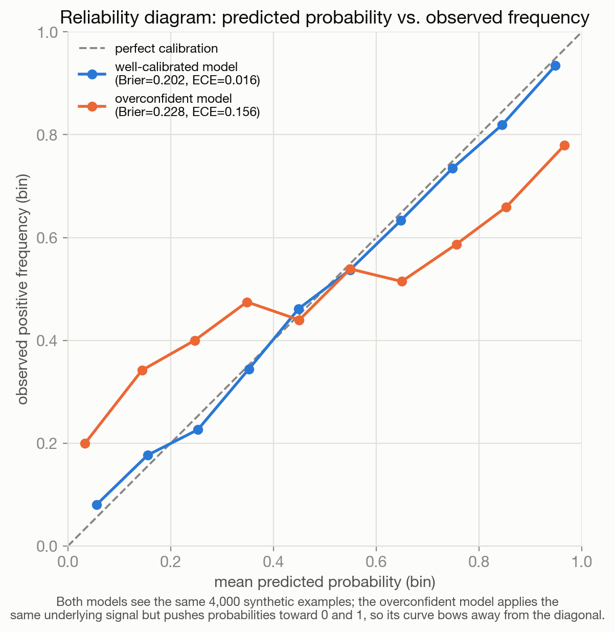
A reliability diagram makes miscalibration visible directly: bin predictions by predicted probability, and for each bin plot the observed frequency of the positive class against the bin’s mean predicted probability. A perfectly calibrated model traces the diagonal \(y=x\) exactly — among examples the model called “80% confident,” 80% should in fact be positive. Figure 16.1 shows this for two synthetic classifiers built from the same 4,000-example ground truth: a well-calibrated model whose curve hugs the diagonal, and an overconfident model — one that takes the same underlying signal and pushes probabilities toward 0 and 1 — whose curve bows visibly away from it, over-predicting near 0 and under-predicting near 1 relative to what actually happens.
Two scalar summaries compress a reliability diagram into a single number. Expected calibration error (ECE) is the weighted average gap between predicted probability and observed frequency across bins:
\[ \mathrm{ECE} = \sum_{b=1}^{B} \frac{|S_b|}{n} \left| \, \overline{p}_b - \overline{y}_b \, \right| \]
where \(S_b\) is the set of examples in bin \(b\), \(\overline{p}_b\) the mean predicted probability in that bin, and \(\overline{y}_b\) the observed positive rate. Brier score is the mean squared error between predicted probability and the binary outcome, \(\frac{1}{n}\sum_i (\hat p_i - y_i)^2\) — it’s a proper scoring rule, meaning it’s uniquely minimized in expectation by reporting your true belief, which is what makes it usable to compare models directly rather than just diagnosing one model’s shape. In the figure, the overconfident model has both a higher Brier score (worse overall probabilistic accuracy) and a much higher ECE (worse calibration specifically) than the well-calibrated one, despite both being built from the identical underlying signal — the only difference is how aggressively each pushes its stated confidence toward the extremes.
If a model is well-calibrated but you need it to be better-calibrated without retraining, standard fixes are Platt scaling (fit a logistic regression from raw scores to calibrated probabilities on a held-out set) or isotonic regression (fit a non-parametric monotonic mapping) — both cheap post-hoc corrections layered on top of an existing model’s scores.
Classification and ranking metrics
Accuracy, precision, recall, F1, ROC-AUC for classification, and nDCG, MRR, and precision@k for ranking are covered in full where they’re the primary object of study — Supervised Learning for the classification metrics and their precision/recall trade-off, and Information Retrieval, Ranking, and Recommenders for the ranking-specific metrics and why accuracy is the wrong lens entirely once output order matters. The point worth making here, rather than re-deriving them, is how they fit into the broader evaluation picture: these are all still offline, held-out metrics, and inherit every caveat above about diverging from what actually matters in production. A ranking model with excellent offline nDCG can still rank content that’s technically relevant but unhelpful, unsafe, or redundant near the top — nDCG only knows about the relevance labels it was given, not the parts of “good” that were never captured in the labeling scheme.
Benchmark contamination and overfitting to leaderboards
A benchmark is only informative if the model being scored on it hasn’t already seen the answers. Contamination happens when benchmark questions (or close paraphrases) end up in a model’s pretraining corpus — easy to happen by accident at internet scale, since benchmark datasets and their solutions are often themselves published on the web — so a high score partly reflects memorization rather than the capability the benchmark meant to measure. This is hard to detect from outside a lab (you generally can’t inspect the pretraining data), and it’s why held-out contamination checks (searching training data for near-duplicates of benchmark items) and benchmarks explicitly built to be refreshed with genuinely novel items are taken increasingly seriously.
Overfitting to a leaderboard is a subtler version of the same problem that doesn’t require literal data leakage. When a benchmark becomes the target that a whole field iterates against — trying architecture and training-recipe variations, keeping the ones that move the number — the benchmark score improves partly by fitting details specific to that benchmark’s particular distribution of question types, phrasing conventions, or scoring quirks, in a way that doesn’t transfer to the broader capability the benchmark was a proxy for. This is Goodhart’s law again, operating at the level of an entire research community rather than a single model. It’s why a single static leaderboard number, however large the benchmark, is a weak signal in isolation, and why serious evaluation practice looks at performance across many benchmarks probing different things, tracks whether gains transfer to genuinely held-out or newly-constructed evaluations, and treats a large jump on one popular benchmark with more skepticism, not less.
Human evaluation
For open-ended generation, many outputs can be acceptable and there’s often no single ground-truth answer to check against, which is exactly the setting where human judgment becomes necessary rather than optional. The methodological core of human evaluation is inter-rater agreement: whether independent human raters, given the same instructions and the same output, converge on the same judgment. Agreement is typically summarized with Cohen’s kappa (two raters) or Fleiss’ kappa (more than two), which correct raw agreement rate for the agreement you’d expect by chance alone — raw agreement can look high purely because most items are easy, so kappa is the more honest number. Low agreement is itself a diagnostic: it usually means the rating instructions are ambiguous, the task genuinely has no consensus answer, or the raters lack the expertise to judge it — any of which should be fixed before trusting the resulting scores, not papered over by averaging across more raters.
Human evaluation is good at judging exactly the properties that are hard to specify as a formula — is this response actually helpful, does this image look right, is this summary faithful to the source, would a real user be satisfied. It’s expensive and slow, though, and it doesn’t scale to per-commit or per-training-step iteration, which is the practical reason automated judges exist at all: not because they’re better than humans at judging quality, but because they’re available at a scale and speed human raters can’t match.
LLM-as-judge
Using one LLM to score another model’s outputs — “LLM-as-judge” — has become a standard evaluation tool precisely because it sits in the gap human evaluation leaves: much cheaper and faster than humans, while still able to assess open-ended qualities that a formula can’t (unlike BLEU/ROUGE-style n-gram overlap metrics, an LLM judge can recognize that a paraphrase is a correct answer). It is not a free substitute for ground truth, though — a judge model has systematic biases worth naming explicitly, because they predict specific, exploitable failure patterns rather than generic noise:
- Position bias: when a judge is shown two candidate responses side by side and asked which is better, it tends to favor whichever one appears in a particular position (often first) more than the content alone justifies. The standard mitigation is running the comparison twice with the order swapped and checking whether the verdict flips.
- Verbosity bias: judges systematically tend to rate longer responses as better, independent of whether the extra length adds real content — an answer padded with restatement and hedging can out-score a shorter, more precise one purely on length. This is the LLM-judge analogue of the reward-hacking problem in RLHF: if verbosity correlates with judged quality, optimizing against the judge (or against a reward model trained from similar judgments) will learn to pad.
- Self-preference bias: a model used to judge outputs — including its own family’s outputs — tends to rate responses written in a style similar to its own generation style more favorably, which becomes a real problem when a lab evaluates its own model using itself (or a close relative) as judge.
Because of these biases, an LLM judge needs to be validated against human judgments before it’s trusted for anything consequential: run the judge and human raters on the same sample of outputs, and check that the judge’s verdicts agree with human verdicts at a level similar to how well independent humans agree with each other. A judge that clears that bar can be trusted to extend human judgment to far more examples than humans alone could rate; a judge that doesn’t clear it is measuring something else — often, specifically, length or surface style — and should not be reported as if it were measuring quality.
Statistical significance and online evaluation
All of the above — offline metrics, calibration, human ratings, LLM-judge scores — are still, at best, well-validated proxies. The actual arbiter of whether a change helps in the way that matters is an online, randomized comparison against real usage: an A/B test. The methodology (randomization, power analysis, avoiding peeking, multiple-comparison correction, the distinction between statistical and practical significance) is developed in full in Causal Inference and Experimentation, since A/B testing is fundamentally a randomized-experiment problem, not a model-evaluation-specific one — the same discipline that validates a drug or a policy change validates a new ranking model or a new prompt. The point worth making here is why it’s the final arbiter rather than just one more metric in the stack: it’s the only one of these methods that measures the actual causal effect of shipping the change on the actual outcome you care about, under real, uncurated traffic, with no proxy or judge standing in between. Every method earlier in this chapter exists to let you iterate fast and cheaply before paying the cost of a real online test — but “the offline metric improved,” “the judge preferred it,” and even “human raters preferred it” are all still hypotheses about what will happen in production, and an A/B test is where that hypothesis actually gets checked.
16.2 Main methods
Put together, a mature evaluation setup for a generative or agentic system in 2026 typically layers several of these rather than picking one:
- Offline held-out metrics (task-appropriate: accuracy/F1 for classification, nDCG for ranking, exact-match or pass@k for verifiable tasks like code and math) for fast, cheap iteration during development.
- Calibration checks wherever a downstream decision consumes a probability or confidence score directly, not just a top prediction.
- Contamination-aware benchmarking: multiple benchmarks, preference for ones refreshed with novel items, explicit skepticism toward suspiciously large single-benchmark jumps.
- LLM-as-judge, validated periodically against a human-rated sample, for scaling open-ended quality assessment beyond what human raters alone could cover.
- Human evaluation on a smaller, carefully sampled set, particularly for high-stakes judgments (safety, factuality in sensitive domains) where judge bias risk is least acceptable.
- Online A/B testing as the final gate before broad rollout, measuring the actual causal effect on the actual product outcome.
16.3 When to use it / what can go wrong
A benchmark score that’s contaminated is worse than no benchmark score at all, because it actively misleads: it looks like rigorous evidence while carrying none of the information it claims to. The practical defense is triangulation — no single number, however precise, should be trusted alone; agreement across offline metrics, human evaluation, and (eventually) online results is the actual signal, and disagreement between them is itself diagnostic information about which proxy is failing.
An LLM judge that just rewards longer answers is not a hypothetical — it’s the default outcome of deploying an unvalidated judge, because verbosity bias is close to universal across judge models unless specifically controlled for (e.g. explicitly instructing the judge to penalize unnecessary length, or controlling for length statistically in the analysis). If a team optimizes a model against such a judge — using judge scores as an RLHF-style reward signal, for instance — the model will learn to be verbose, the judge score will climb, and the model will get worse at the thing users actually wanted, all while the reported metric goes up. This is exactly the metric-proxy divergence from the opening section, just wearing an LLM-judge costume instead of a classic offline-metric one.
A calibration check that’s skipped is a subtler trap: a model can pass every accuracy-style benchmark while being badly overconfident, and that failure only shows up once the probabilities themselves are used for something — risk thresholds, human-review triage, an agent’s decision about when to ask for help versus act autonomously. Since accuracy and calibration are different axes, good accuracy is no evidence at all about calibration one way or the other, and needs to be checked directly rather than assumed.
Finally, running an A/B test underpowered, or stopping it early the moment it looks favorable (“peeking”), inflates the false-positive rate well beyond the nominal significance threshold — a change that looks statistically significant on day 2 of a planned two-week test is far more likely to be noise than the same result observed at the test’s planned conclusion. This and other experimentation pitfalls are covered in depth in Causal Inference and Experimentation.
16.4 How this connects
- Supervised Learning — precision, recall, ROC-AUC, and the bias-variance framing of generalization are the classification-metric foundation this chapter points back to rather than re-deriving.
- Information Retrieval, Ranking, and Recommenders — nDCG, MRR, and precision@k are defined there in full, and inherit the same offline/online divergence concerns developed here.
- Generative AI and Foundation Models — factuality, groundedness, helpfulness, and diversity are exactly the properties generative model evaluation needs beyond raw likelihood, and are assessed with the human/LLM-judge machinery developed here.
- AI Agents, Tool Use, and Multi-Agent Systems — evaluating an agent means evaluating a whole trajectory’s success, not a single response, which raises the stakes on getting judge validation and online testing right rather than trusting a single offline proxy.
- Causal Inference and Experimentation — A/B testing methodology (randomization, power, significance, peeking) is developed in full there; this chapter treats it as evaluation’s final arbiter rather than repeating the statistics.
- Conformal Prediction — where calibration in this chapter is about probabilities matching frequencies on average, conformal prediction gives a distribution-free, finite-sample coverage guarantee for prediction sets, a complementary and stronger kind of reliability guarantee.