6 Graphical Models and Latent Variables
Real systems of random variables rarely come in pairs. A recommender system has millions of users and items whose ratings all depend on each other through shared latent taste; a diagnosis system has symptoms, test results, and diseases where each symptom depends on the disease but not directly on the test results; a sequence of user actions has today’s state depending on yesterday’s but not, given yesterday’s, on last week’s. Writing out a full joint distribution over dozens or millions of variables by brute force is hopeless — a joint distribution over \(n\) binary variables has \(2^n\) entries. Graphical models solve this by using a graph to declare, explicitly and compactly, which variables directly influence which others, so that the full joint distribution factors into small, local, tractable pieces. Latent variable models solve a related but different problem: often the variables you can actually observe (words in a document, ratings in a matrix, pixels in an image) are not the ones that generated the interesting structure — a hidden topic, a hidden taste vector, a hidden cluster — and you need a principled way to reason about a variable you never get to see directly. These two ideas combine constantly in practice, because most useful latent variable models are most cleanly expressed as a graphical model with some of its nodes shaded “unobserved.”
6.1 How it works
Graphs as compact factorizations
The chain rule of probability lets you factor any joint distribution as a product of conditionals: \(p(x_1, \ldots, x_n) = \prod_i p(x_i \mid x_1, \ldots, x_{i-1})\). That’s always true but useless on its own, because the \(i\)-th conditional can depend on all \(i-1\) variables before it, and the number of parameters needed to specify that grows exponentially. A Bayesian network is a directed acyclic graph where each node’s conditional distribution depends only on its graph parents, not on every variable that precedes it in some arbitrary ordering:
\[ p(x_1, \ldots, x_n) = \prod_{i=1}^n p(x_i \mid \mathrm{parents}(x_i)) \]
This factorization is a genuine assertion about the world — it claims that, given its parents, each variable is conditionally independent of its non-descendants. A patient’s test result depends on whether they have the disease, not directly on which symptoms they happen to have reported; encoding that as an edge structure (disease → test result, disease → symptoms, but no symptom → test-result edge) turns an intractable joint distribution over all variables into a product of small, locally specified conditional probability tables, each of which needs only as many parameters as its node has parents, not the whole variable set.
Markov random fields use undirected edges instead, and are the natural choice when the dependency between two variables isn’t naturally causal or directional — adjacent pixels in an image tend to have similar values, but neither pixel “causes” the other; two neighboring words in a sentence constrain each other symmetrically. Rather than conditional probability tables, an MRF factors the joint as a product of non-negative potential functions over cliques (fully connected subsets) of the graph, normalized by a partition function:
\[ p(x_1, \ldots, x_n) = \frac{1}{Z}\prod_{c \in \mathrm{cliques}} \psi_c(x_c) \]
The potentials \(\psi_c\) don’t need to be probabilities themselves — just non-negative compatibility scores, high when the clique’s variables agree with each other in a way the model favors — and \(Z\), the sum or integral of the numerator over every possible configuration, renormalizes the whole thing into a valid distribution. \(Z\) is usually intractable to compute exactly for anything but small or specially structured graphs, which is a recurring theme this entire chapter and the next one keep bumping into.
Factor graphs make the factorization itself an explicit, first-class object: a bipartite graph with one type of node for variables and another for the factors (the individual conditional probabilities or potential functions) connecting them, with an edge whenever a factor’s function depends on that variable. This representation unifies Bayesian networks and MRFs under one picture and is the natural substrate for message-passing inference algorithms (belief propagation), which compute exact marginals efficiently by passing local messages along the graph whenever the graph happens to be a tree — and approximate marginals, with no such guarantee but often useful results in practice, when it isn’t.
Conditional independence is an assumption, not a fact
Every edge you draw and every edge you omit is a claim. Omitting the edge between two variables is the assertion that they are conditionally independent given their parents (in a Bayesian network) or given their Markov blanket (in an MRF) — and that assertion is what buys you the tractable factorization above. This is genuinely useful: it’s what makes inference computationally feasible at all, and a well-chosen structure often reflects real, defensible domain knowledge (a test result really is only informative about a disease, not independently about unrelated symptoms). But it is a modeling choice, not a law of nature, and it can be wrong in ways that matter — assuming two variables are conditionally independent when they’re actually correlated even after conditioning will bias any inference drawn from the model, sometimes badly. Naive Bayes, from the previous chapter, is the starkest example: it assumes every feature is conditionally independent given the class, which is almost never literally true, and yet the model is often still useful because the decision boundary it induces degrades gracefully even when the independence assumption is violated. The lesson generalizes: treat the graph structure as a hypothesis about the data generating process, one you can and should sanity-check against domain knowledge and, where possible, against the data itself.
Latent variables and the EM algorithm
A latent variable is one that participates in the generative story but is never observed — a hidden cluster label, a hidden topic assignment, a hidden user preference vector. The trouble with fitting a model that has latent variables by direct maximum likelihood is that the likelihood you’d need to maximize requires marginalizing (summing or integrating) over every possible value of the hidden variable, which usually turns a nice log-likelihood into an intractable log of a sum:
\[ \log p(x \mid \theta) = \log \sum_z p(x, z \mid \theta) \]
The log of a sum has no clean derivative in \(\theta\) the way a sum of logs would, which is exactly what you’d get if \(z\) were observed. The Expectation-Maximization (EM) algorithm sidesteps this by alternating between two easier subproblems instead of solving the hard one directly:
- E-step: given the current parameters \(\theta^{(t)}\), compute the posterior distribution over the hidden variable for each data point, \(p(z \mid x, \theta^{(t)})\) — a soft, probabilistic guess at what the hidden variable’s value probably is, given what’s been observed and the current model.
- M-step: update the parameters to maximize the expected complete-data log-likelihood, \(\mathbb{E}_{z \sim p(z\mid x,\theta^{(t)})}[\log p(x, z \mid \theta)]\), treating the E-step’s soft assignments as if they were real (fractional) observed data.
Each full EM iteration is provably guaranteed to never decrease the true marginal log-likelihood \(\log p(x \mid \theta)\) — the reason is that the E-step’s expected complete-data log-likelihood is a tight lower bound (touching at \(\theta^{(t)}\)) on the true log-likelihood, so maximizing that lower bound in the M-step can only push the true objective up or leave it unchanged, never down. This is why EM is useful whenever direct maximum likelihood is intractable because of a hidden variable, but the conditional subproblems (infer \(z\) given \(\theta\); fit \(\theta\) given a soft assignment of \(z\)) are each individually easy — which is precisely the situation with mixture models, HMMs, and many matrix factorization variants. What EM does not guarantee is convergence to the global maximum: the objective it’s climbing is generally non-convex, so different parameter initializations can land in different local optima, which is why practical implementations restart EM from several random initializations and keep the best result.
A worked example: fitting a Gaussian mixture with EM
Concretely, for a Gaussian mixture model with \(K\) components, the E-step computes, for every point \(x_i\) and every component \(k\), the posterior probability (called the responsibility) that component \(k\) generated \(x_i\):
\[ \gamma_{ik} = p(z_i = k \mid x_i, \theta^{(t)}) = \frac{\pi_k \, \mathcal{N}(x_i \mid \mu_k, \Sigma_k)}{\sum_{j=1}^K \pi_j \, \mathcal{N}(x_i \mid \mu_j, \Sigma_j)} \]
— literally Bayes’ rule applied to the current mixture parameters, treating the hidden cluster label as the unknown. The M-step then re-estimates each component’s mean, covariance, and mixing weight as responsibility-weighted versions of the ordinary Gaussian MLE formulas:
\[ \mu_k = \frac{\sum_i \gamma_{ik}\, x_i}{\sum_i \gamma_{ik}}, \qquad \Sigma_k = \frac{\sum_i \gamma_{ik} (x_i - \mu_k)(x_i - \mu_k)^\top}{\sum_i \gamma_{ik}}, \qquad \pi_k = \frac{1}{n}\sum_i \gamma_{ik} \]
Every point contributes to every cluster’s parameters, weighted by how plausible it is that the point belongs there — a soft, probabilistic version of the hard, one-cluster-per-point assignment that k-means makes. Iterating E- and M-steps drives the responsibilities toward a stable partition of the data and settles each Gaussian onto one of the underlying clusters, as shown in Figure 6.1 on synthetic 2D data from three true clusters with distinct shapes.
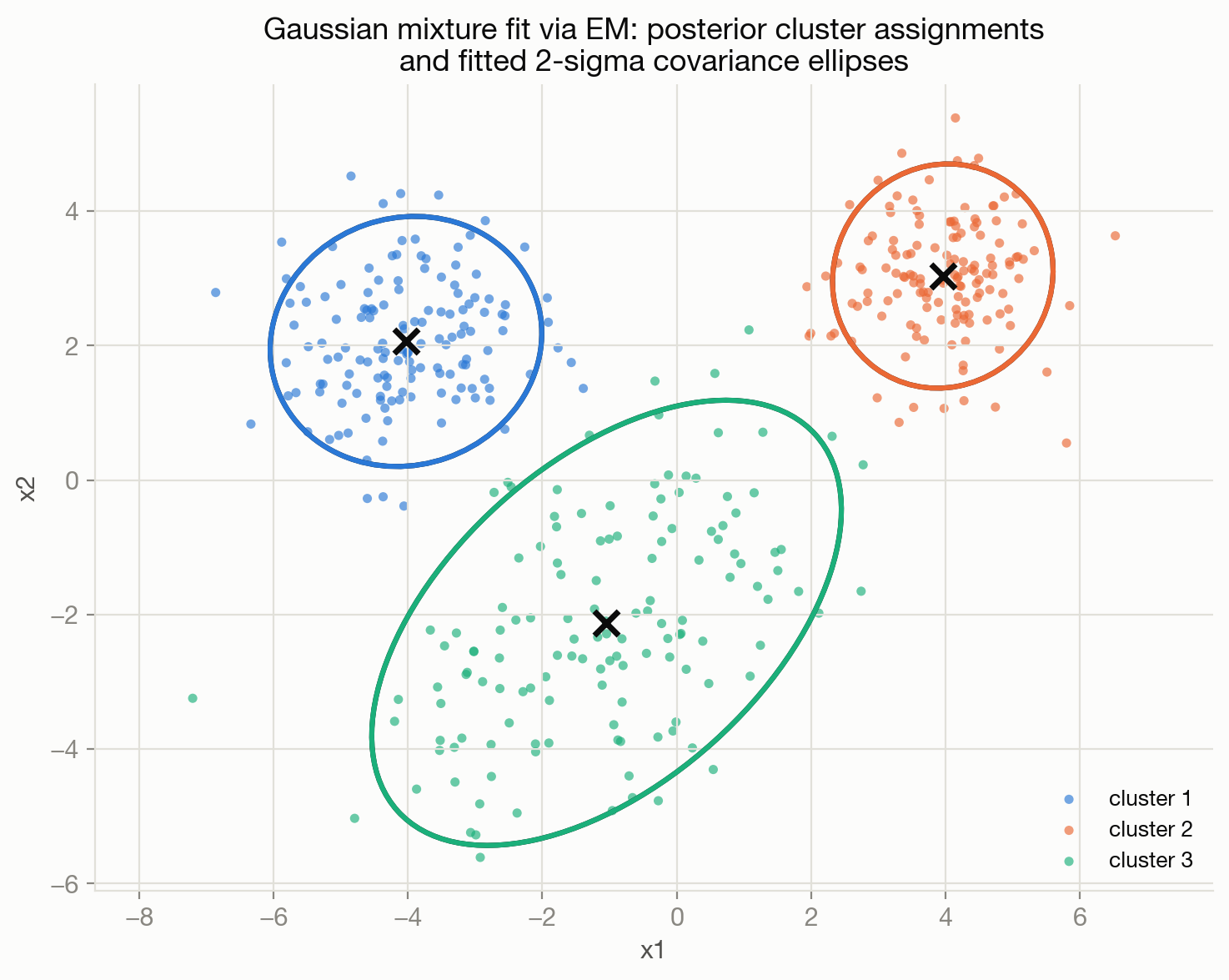
The fitted ellipses tracking the true cluster shapes, including the sheared one, is the concrete payoff of modeling \(\Sigma_k\) as a full covariance matrix rather than assuming isotropic clusters: EM recovers not just where each cluster is centered but its actual shape and orientation, purely from the responsibility-weighted statistics above, with no cluster-shape assumption baked in beyond “Gaussian.”
6.2 Main methods
Mixture models. The general pattern behind the GMM example: each observation is generated by first drawing a hidden component/cluster label, then drawing the observation from that component’s distribution. The components don’t have to be Gaussian — mixtures of Bernoullis, Poissons, or categorical distributions follow the identical EM recipe, just with the component-specific MLE formulas swapped in for the M-step.
Hidden Markov Models (HMMs). Extend the mixture-model idea across time: a hidden state evolves according to a Markov chain (each state depends only on the previous one), and at each time step the hidden state emits an observation according to a state-specific distribution. The hidden state sequence is never observed directly, only the emissions are — used for speech recognition, part-of-speech tagging, and any sequential process where an unobserved regime (a market state, a user’s task-in-progress) drives observable behavior. Fitting an HMM’s parameters from only the emissions is done with the Baum-Welch algorithm, which is EM specialized to this chain structure, using the forward-backward algorithm’s dynamic-programming recursions in place of the plain E-step formula above.
Topic models. As introduced in the previous chapter, Latent Dirichlet Allocation treats each document as a mixture over hidden topics and each topic as a distribution over words, with both the per-document topic mixture and the per-word topic assignment latent. Exact EM is intractable here because the posterior over the full assignment doesn’t factor cleanly, which is why LDA is typically fit with variational inference or collapsed Gibbs sampling instead of vanilla EM — a preview of the approximate-inference machinery the next chapter covers in depth.
Matrix factorization. Explains an observed user-item interaction matrix (ratings, clicks, purchases) as the product of low-dimensional hidden user and item factor vectors, \(r_{ui} \approx u_u^\top v_i\). The hidden factors are latent variables in exactly the sense of this chapter — never observed, only inferred from the pattern of interactions — and the probabilistic version from the previous chapter fits naturally into an EM-like alternating scheme (fix item vectors, solve for user vectors in closed form; fix user vectors, solve for item vectors; repeat), which is the classical alternating least squares algorithm for large-scale recommender systems.
Variational Autoencoders (VAEs). The neural-network extension of this whole framework: a latent variable model where both the generative model \(p(x \mid z)\) and an approximate posterior \(q(z \mid x)\) are parameterized by neural networks, trained jointly by maximizing a tractable lower bound on the log-likelihood (the ELBO) rather than by EM directly, because with a neural-network likelihood the E-step’s exact posterior is no longer available in closed form. The “amortized inference” in a VAE — training a single network \(q(z\mid x)\) that maps any \(x\) straight to an approximate posterior, instead of solving a fresh inference problem for every data point — is the scalable answer to exactly the intractability that motivated alternatives to the “recompute an exact posterior every E-step” version of EM used above.
6.3 When to use it / what can go wrong
Reach for a graphical or latent-variable model when the problem has real structure worth encoding explicitly — known conditional independencies, a believable hidden mechanism (a cluster, a topic, a regime, a taste vector) that explains correlations in what you actually observe — and when you want that structure to buy you either interpretability (a graph you can inspect and reason about) or statistical efficiency (fewer parameters than a fully general joint distribution would require).
Wrong number of latent components. Mixture models and topic models require you to choose \(K\) up front, and getting it wrong in either direction causes real damage: too few components forces the model to merge genuinely distinct clusters into one, blurring the compromise between them; too many lets the model split one true cluster into fragments or overfit noise into spurious extra clusters. Model-selection criteria (BIC, cross-validated held-out likelihood) or nonparametric alternatives (Dirichlet process mixtures, which let the effective number of components grow with the data) are the standard mitigations, but neither replaces sanity-checking the result against domain knowledge.
Local optima. EM (and most latent-variable fitting more generally) only guarantees convergence to a stationary point of a generally non-convex objective, not the global optimum — the algorithm can and does get stuck in different, sometimes badly suboptimal solutions depending on initialization. Always run from multiple random restarts and keep the best (highest likelihood) result, and be suspicious of a single EM run’s output presented without that check.
A wrong graph structure produces confidently wrong inferences. Because conditional independence assumptions are what make the whole factorization tractable, they’re easy to bake in implicitly and forget to question. If two variables you’ve modeled as conditionally independent are actually correlated given their parents, every downstream marginal and every inference drawn from the model can be systematically biased, and — unlike an obviously bad point prediction — a badly structured graphical model can still produce plausible-looking, confidently stated probabilities that are simply wrong. Structure learning algorithms and domain-expert review are both worth investing in before trusting a hand-specified graph at any real scale.
Latent variables are not automatically meaningful. A fitted topic or cluster is a mathematical artifact of the model and the objective it optimized, not a guarantee that it corresponds to a real, semantically coherent concept a human would recognize. Always inspect what the latent structure actually captures (top words per topic, example members per cluster) before treating it as ground truth for a downstream product decision.
6.4 How this connects
- Probabilistic Modeling supplies every primitive this chapter builds with — Bayes’ rule, likelihoods, conjugate updates — and the Gaussian mixture model derived above is the direct latent-variable extension of that chapter’s Naive Bayes and GMM introduction.
- Sampling and Approximate Inference is where you go the moment EM’s exact E-step becomes intractable (as it already is for LDA above) — MCMC and variational inference are the general toolkit for posteriors that have no closed form.
- Representation Learning picks up exactly where VAEs left off: learned latent representations as a general-purpose tool for downstream tasks, not just as a component of a generative model.
- Sequence, Time-Series, and State Models generalizes the HMM’s hidden-state-evolving-over-time idea to richer dynamics (RNNs, state space models), trading the HMM’s exact tractable inference for greater representational flexibility.
- Information Retrieval, Ranking, and Recommenders depends directly on the matrix factorization latent-variable model described above as one of the core techniques for learning user and item representations from sparse interaction data.