13 Information Retrieval, Ranking, and Recommenders
Almost every system that shows a person a small, ordered list drawn from a much larger collection — search results, a product feed, a music queue, a newsfeed — is solving the same three-stage problem, even though the stages are usually invisible from the outside. First, retrieval: given a query (explicit, like a search term, or implicit, like “this user, right now”), find a manageable set of candidates from a collection that might be millions or billions of items — too large to score every item individually within a latency budget. Second, ranking: order that candidate set by predicted relevance, using a model expensive enough to be accurate but cheap enough to run on the (now much smaller) candidate set. Third, re-ranking: adjust the ranked list for concerns beyond raw relevance — diversity, freshness, business rules, safety filters — before it’s actually shown. Recommender systems are this same pipeline personalized: retrieval and ranking conditioned not just on an explicit query but on a specific user’s history, context, and inferred preferences. The reason this decomposition exists at all, rather than one model doing everything end to end, is a hard computational constraint: the most accurate scoring functions are usually too expensive to run against every item in the collection, so cheaper, coarser methods are used to cut the collection down before the expensive model ever runs.
13.1 How it works
Retrieval: narrowing millions down to hundreds
Retrieval has to answer “which items could plausibly be relevant” cheaply enough to run against the entire collection. Three broad families:
Lexical retrieval matches query terms against document terms directly, using an inverted index (a mapping from each term to the list of documents containing it) so that finding “documents containing this word” is a fast lookup rather than a scan. BM25 is the standard scoring function on top of that index: it scores a document for a query by summing, over query terms present in the document, a term-frequency-weighted score that saturates (diminishing returns for repeated occurrences of the same term — the tenth occurrence of a word shouldn’t count nearly as much as the first) and is down-weighted for terms that appear in many documents across the collection (inverse document frequency — a term that’s rare across the collection is more informative when it does appear) and normalized for document length (so a long document doesn’t win purely by containing more words). This is fast, interpretable, requires no training, and is extremely hard to beat on exact keyword and rare-term matching — but it has no notion of meaning: a query for “automobile” will not match a document that only says “car.”
Dense retrieval solves exactly that gap by embedding queries and documents into a shared vector space (typically with a Transformer encoder — see Deep Learning Foundations and Representation Learning) such that relevant query-document pairs land close together, usually trained with a contrastive objective that pulls known-relevant pairs together and pushes random or hard-negative pairs apart. At serving time, finding the nearest document vectors to a query vector across millions or billions of documents is itself a nontrivial computational problem, solved with approximate nearest neighbor (ANN) search (HNSW graphs, IVF with product quantization, and similar structures) that trade a small amount of recall for orders of magnitude in speed compared to exact nearest-neighbor search. Dense retrieval captures semantic similarity that lexical matching structurally cannot, but it can miss exact rare-term matches (a product SKU, a legal citation, a person’s name) that BM25 would catch trivially, and it requires training data and infrastructure that lexical retrieval doesn’t.
Hybrid retrieval combines both — typically by taking the union of candidates from a lexical index and a dense ANN index, then combining or re-scoring, sometimes with a simple linear blend of the two scores, sometimes by feeding both signals into a downstream ranker. In practice this is close to a default choice in production search systems specifically because lexical and dense retrieval fail on almost disjoint sets of queries — lexical retrieval is weak on semantic/paraphrase queries, dense retrieval is weak on exact rare-term queries — so the union recovers most of both methods’ strengths.
Ranking: ordering candidates by predicted relevance
Once a candidate set is small enough (hundreds, not millions), a more expensive model can score every candidate. How that scoring is framed as a learning problem is a real design choice with real tradeoffs:
- Pointwise ranking treats each (query, document) pair independently and trains a regressor or classifier to predict its relevance score directly — simple to implement and train with standard supervised-learning tools, but it optimizes the wrong thing: getting every individual relevance estimate slightly wrong in a way that preserves relative order costs nothing to the end user, while getting the order wrong for even one pair does, and pointwise loss doesn’t distinguish between those two failure modes.
- Pairwise ranking instead trains on the relative order of pairs of documents for the same query — the model just needs to get “A should rank above B” right, not the absolute score of either. RankNet and LambdaMART (a pairwise-trained gradient-boosted tree ranker, directly building on the gradient boosting machinery in Trees, Ensembles, and Tabular ML) are the classic examples, and LambdaMART in particular remains a strong, widely deployed production baseline because it directly incorporates a ranking-metric-aware weighting into its gradient updates — pair swaps near the top of the ranking are weighted more heavily than swaps far down the list, since that’s where ranking-quality metrics like nDCG are most sensitive.
- Listwise ranking optimizes an objective over the whole ranked list at once — directly approximating a ranking metric like nDCG rather than a proxy pairwise or pointwise loss. This is the closest match to what’s actually being evaluated, but the true ranking metrics are non-differentiable (they depend on sort order, which has zero gradient almost everywhere), so listwise methods have to use a smooth surrogate (e.g. ListNet’s probabilistic relaxation of a permutation, or LambdaMART’s metric-weighted pairwise gradients, which sit somewhere between pairwise and listwise in spirit).
- Reranking is the final adjustment pass applied after a relevance-based ranking: diversity (don’t show ten near-duplicate results), freshness (boost recent content when recency matters), safety/policy filtering, and business constraints (inventory, contractual placement requirements). This is deliberately kept as a separate stage rather than folded into the relevance model because these objectives change faster and more situationally than “what is relevant,” and because they’re often easier to reason about and audit as explicit rules or a lightweight adjustment layer than as an entangled part of a single opaque scoring function.
Recommenders: personalizing both stages
A recommender system runs the same retrieval-then-ranking pipeline, but conditions it on a specific user rather than (or in addition to) an explicit query.
Collaborative filtering predicts a user’s preference for an item based on patterns across many users’ preferences, on the premise that users who agreed in the past will tend to agree in the future — no content understanding of the items required at all. Matrix factorization is the classic realization: represent the (sparse, mostly-unobserved) user-item interaction matrix \(R\) as the product of two low-rank matrices, \(R \approx U V^\top\), where each row of \(U\) is a learned user embedding and each row of \(V\) is a learned item embedding, trained to reconstruct observed interactions (with regularization, since most entries are missing rather than zero — the model is asked to predict entries it never saw, not to reconstruct a fully observed matrix). This is directly a latent-variable model in the sense developed in Graphical Models and Latent Variables: the embeddings are unobserved variables inferred to explain observed co-occurrence patterns, learned essentially the same way factor analysis or probabilistic matrix factorization would frame it, just usually fit by direct gradient-based optimization of reconstruction error (plus regularization) rather than full posterior inference.
Content-based recommendation goes the other way: predict preference from item and user features directly (genre, text, image embeddings, declared interests) rather than from cross-user interaction patterns. It has no cold-start problem for new items with known features, but it can’t discover that two items are related in ways their surface features don’t capture — exactly the complementary blind spot to collaborative filtering’s blind spot on new items and new users with no interaction history yet.
Two-tower retrieval is the dominant architecture for the retrieval stage of a modern personalized system: one neural tower encodes the user (and context) into an embedding, a separate tower encodes each item into an embedding in the same space, and the two are trained jointly (again typically with a contrastive loss) so that relevant user-item pairs land close together. Structurally this is dense retrieval’s query/document towers specialized to users and items, and it has the same appeal: at serving time, item embeddings are precomputed once, and finding a user’s best candidate items is exactly the ANN nearest-neighbor search problem again — the two-tower architecture is popular specifically because it decouples user and item computation in a way that makes large-scale approximate retrieval possible.
Deep ranking models take the small candidate set produced by retrieval (two-tower or otherwise) and score it with a heavier model that can use rich cross-features between user and item — attention over a user’s interaction history, wide-and-deep architectures combining memorization and generalization, feature crosses that a two-tower architecture’s independent-encoding structure cannot represent (since a two-tower model never lets user and item features interact until the final dot product, which is exactly the computational property that makes it fast at retrieval-time scale, and exactly the representational limitation that makes it too weak for final ranking).
Sequential recommendation treats a user’s interaction history as an ordered sequence and predicts the next item using sequence models (RNNs, 1D convolutions, or — increasingly — Transformer-style self-attention over the interaction sequence), directly borrowing the machinery from Sequence, Time-Series, and State Models. This captures short-term intent and session dynamics (what you just looked at strongly predicts what you want next) that a static user embedding averages away.
Bandit-based exploration in recommenders addresses a problem the above methods don’t solve on their own: a model trained purely on historical interaction data will keep recommending what already performed well historically and will systematically undertest new or under-shown items, which is exactly the exploration-exploitation problem covered in Reinforcement Learning and Bandits. Treating candidate items as bandit arms (often contextual, with the user as context) gives a principled way to allocate some traffic to under-tested-but-potentially-good items rather than purely exploiting historical performance.
Metrics
Retrieval and ranking quality need different metrics because they’re answering different questions. Recall@K (of all truly relevant items, how many are in the top K) is the standard retrieval-stage metric — it doesn’t care about order within the top K, because retrieval’s job is just to make sure relevant items survive to the ranking stage, not to order them. MRR (mean reciprocal rank — the reciprocal of the rank position of the first relevant result, averaged over queries) suits tasks where only the first relevant hit matters, like navigational search or question answering. nDCG@K (normalized discounted cumulative gain) is the standard ranking metric for graded relevance (not just relevant/irrelevant, but relevance on a 0-3 or similar scale): it sums each item’s relevance gain, discounted logarithmically by its rank position (so a highly relevant item at position 1 contributes much more than the same item at position 10), then normalizes by the score of the ideal (perfectly sorted) ranking, so a score of 1.0 always means “as good as possible given these relevance labels regardless of scale.” MAP (mean average precision) averages precision computed at every position where a relevant item appears, which rewards concentrating relevant items near the top across the whole list. Beyond ranking-quality metrics, production systems track CTR, conversion, and retention as business-outcome proxies, and diversity and novelty explicitly, because a ranking system optimized purely for predicted relevance or engagement will systematically converge toward safe, popular, already-known items unless something explicitly counteracts that pull.
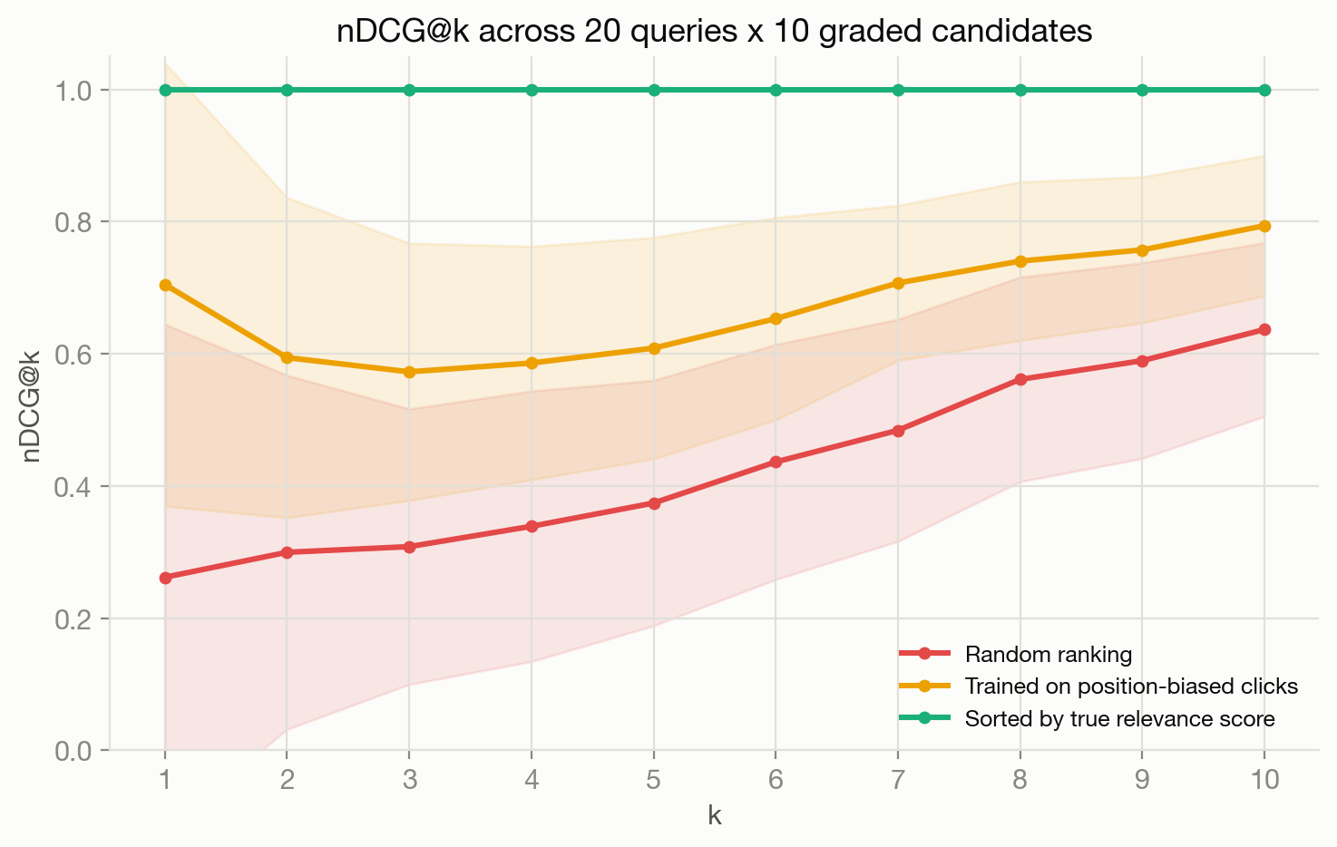
Figure 13.1 makes concrete why nDCG in particular is the standard ranking-quality metric rather than something simpler: it shows nDCG@k computed across 20 synthetic queries, each with 10 graded candidates, for three rankings — random (which should and does score worst and noisiest), a ranking sorted directly by the ground-truth relevance-generating score (which achieves nDCG = 1.0 at every k by construction, since it is the ideal ranking used to normalize the metric), and a ranking trained on a position-bias-corrupted signal, described next.
13.2 When to use it / what can go wrong
Debugging a bad recommendation or search result. When a system surfaces something clearly wrong, the failure could be at any of several distinct points, and they require different fixes:
- Missing candidates. If the right item was never in the candidate set retrieval produced, no amount of ranking-model improvement will ever surface it — this is a retrieval-recall problem, not a ranking problem, and it’s worth checking Recall@K specifically before assuming the ranker is at fault.
- Poor ranking. The right items were retrieved but ordered badly — usually a sign the ranking model’s features or training objective don’t capture what actually matters for this query/user, or that pointwise training is being asked to do a pairwise/listwise job.
- Biased labels. As shown in the figure, if the training signal itself (typically implicit feedback like clicks) reflects what users were shown more than what they actually prefer, the model will learn to reinforce whatever ranking generated the training data in the first place — a self-reinforcing feedback loop. Position bias (users click what’s shown near the top regardless of true relevance, simply because that’s what they see) is the most common instance and needs explicit correction — inverse propensity weighting, randomized exploration in a small slice of traffic to get unbiased labels, or counterfactual learning-to-rank methods that model the exposure process directly rather than treating clicks as ground truth.
- Over-personalization. A system that leans too hard on a user’s past behavior can trap them in a narrow filter bubble, fail to adapt when their interests genuinely shift, and hurt exactly the diversity and discovery metrics that don’t show up in short-horizon engagement numbers.
- Cold start. New users (no interaction history for collaborative filtering to use) and new items (no interaction data for collaborative filtering, but content-based signals may still work) need explicit fallback strategies — content-based scoring, popularity priors, or bandit-driven exploration — since the core collaborative signal simply doesn’t exist yet for them.
- Serving constraints. Latency budgets, index staleness, or infrastructure limits can silently truncate what retrieval even considers (e.g. an ANN index that hasn’t been rebuilt since a new item was added, or a candidate generator that caps at a small K for latency reasons) — a purely model-quality investigation can miss this entirely if nobody checks what the serving system actually had available.
What can go wrong more generally. Optimizing hard for a single short-horizon engagement metric (CTR, watch time) without diversity or long-term-satisfaction guardrails reliably produces the filter-bubble, clickbait-favoring failure mode — the metric gets better while the thing it was meant to proxy for gets worse, a specific instance of Goodhart’s law that recommender teams re-learn often enough that it’s worth designing against from the start, not discovering after the fact. Evaluating a ranking or retrieval change purely offline (on logged data) without an online experiment can also mislead badly, precisely because offline metrics are computed against a fixed, historically-biased label distribution — the same distributional-shift concern that shows up in offline RL — which is why mature ranking teams treat offline metrics as a screening step and trust online A/B experiments for the actual launch decision.
13.3 How this connects
- Reinforcement Learning and Bandits — bandit algorithms are the standard tool for ranking exploration and cold-start item discovery, treating “which item to show” as an exploration-exploitation problem rather than a purely supervised one.
- Graphical Models and Latent Variables — matrix factorization is a latent-variable model of the user-item interaction matrix, and the probabilistic-matrix-factorization view of collaborative filtering makes the connection to full Bayesian latent factor models explicit.
- Graph Neural Networks and Structured Data — large-scale candidate generation increasingly treats the user-item interaction log as a bipartite graph and uses inductive GNNs (e.g. GraphSAGE-style sampling) to produce item embeddings for retrieval, rather than pure matrix factorization.
- Causal Inference and Experimentation — position bias and other forms of exposure-driven label bias are a concrete instance of confounding, and the fix (propensity weighting, randomized exploration) is directly the causal-inference toolkit applied to ranking data.
- Generative AI and Foundation Models — retrieval-augmented generation (RAG) is exactly the retrieval stage described here, feeding retrieved context into a generative model instead of (or in addition to) a ranked list shown directly to a user.