19 ML Systems and MLOps

Training a model that scores well on a held-out set is the easy part of machine learning in production. The hard part — the part that consumes most of the engineering effort in any real system — is turning that model into something that keeps working: fed with fresh, correctly-labeled data; served fast enough and reliably enough for whatever consumes it; watched closely enough that a regression is caught before it does damage; and owned by someone who can act when it breaks. Most of what goes wrong in production machine learning has nothing to do with the model’s architecture or its offline accuracy. It’s data pipelines quietly changing shape, training and serving code disagreeing about what a feature means, a label definition drifting, or a dependency silently failing upstream. ML systems and MLOps is the discipline of building around a model so these failures are visible, attributable, and recoverable, instead of showing up three weeks later as “the metrics just got worse and nobody knows why.”

19.1 How it works

A production ML system is best understood as a loop, not a pipeline with a start and an end. Data flows in, a model is trained and evaluated, it’s promoted to serve live traffic, its predictions get logged, those logs (often combined with delayed outcome data) become the labels for the next training run, and the cycle repeats — usually with humans and automated checks gating each transition. Each stage in that loop is a place where something silent can break:

Data ingestion pulls raw events or records from upstream systems. If an upstream schema changes, or an upstream service silently drops a fraction of events, ingestion is often the first place the damage happens and the last place anyone looks, because the pipeline doesn’t crash — it just quietly serves worse data.
Label generation turns raw events into training targets, which is often the least mechanical, most assumption-laden step in the whole loop: what counts as a “click,” how long to wait before treating a sale as a conversion, how to attribute a delayed outcome back to the prediction that caused it. A label definition change is functionally a silent redefinition of the prediction task, and it can invalidate historical training data without anyone editing a line of model code.
Feature pipelines compute the inputs the model actually sees. This is the single most common source of a specific, insidious bug: train/serve skew, where the feature computed offline during training (often in a batch job with access to future context, or computed slightly differently in Python vs. the production serving language) doesn’t match the feature computed online at serving time. A model can be excellent offline and mysteriously bad online purely because the two code paths that build the same “feature” disagree.
Training, evaluation, and the model registry are where a candidate model is fit, checked against held-out and slice-level metrics, and versioned with enough metadata (training data snapshot, code version, metrics, approval) to make every production model reproducible and auditable after the fact.
Serving exposes the model to real traffic, batch or online, with its own constraints: latency budgets, throughput, hardware cost, and fallback behavior when the model or a dependency is unavailable.
Logging and monitoring record what the model actually predicted, on what inputs, and (once available) what actually happened — the raw material for both debugging and the next round of training data.
Retraining and rollback close the loop: retraining incorporates fresh data (and ideally corrects for whatever drift monitoring caught), and rollback is the escape hatch when a newly promoted model turns out to be worse in ways offline evaluation didn’t catch.

Feedback loops deserve special mention because they’re a failure mode specific to systems that act on their own predictions. If a recommender’s predictions influence what content gets shown, and future training data is drawn from what got shown, the model’s own past predictions shape the data it will be trained on next — an implicit form of confounding that isn’t about a single feature but about the entire training distribution. A model that predicts engagement and gets deployed will, if unchecked, drift toward recommending whatever it already believes is engaging, whether or not that belief was ever accurate, simply because it never sees outcomes for the things it chose not to show. This is the same core problem the exploration side of Reinforcement Learning and Bandits exists to solve, and it’s why production recommender and ranking systems usually need some form of deliberate exploration or logging of counterfactual (not-shown) outcomes to avoid quietly poisoning their own training data.

19.2 Main failure modes

Data drift is a change in the distribution of the model’s input features between training time and the present. Label drift is the analogous change in the distribution of the target itself — user behavior, fraud patterns, or the phenomenon being predicted genuinely shifts over time, independent of any pipeline bug. Both are usually gradual rather than sudden, which is precisely what makes them dangerous: nothing crashes, no alert fires from a hard error, and by the time an aggregate business metric moves enough for a human to notice, the model may have been degrading for weeks.

Detecting drift quantitatively means comparing a reference distribution (usually the training-time distribution of a feature) against a current window, using a statistic sensitive to distributional change. Two common ones:

The Kolmogorov–Smirnov (KS) statistic is the maximum distance between the empirical cumulative distribution functions of the reference and current samples — simple, nonparametric, and sensitive to shifts anywhere in the distribution’s shape.
The Population Stability Index (PSI) bins the reference distribution into quantile buckets, then compares the fraction of the current sample falling in each bucket against the reference fraction: \[ \text{PSI} = \sum_{i} (\text{cur}_i - \text{ref}_i) \, \ln\!\left(\frac{\text{cur}_i}{\text{ref}_i}\right), \] summed over bins \(i\). PSI values below roughly 0.1 are usually treated as no meaningful shift, 0.1–0.2 as a moderate shift worth watching, and above 0.2 as a shift that typically warrants investigation or retraining — thresholds that are conventions from the credit-risk industry, not laws of nature, and worth calibrating against how sensitive a given feature and model actually are to shift.

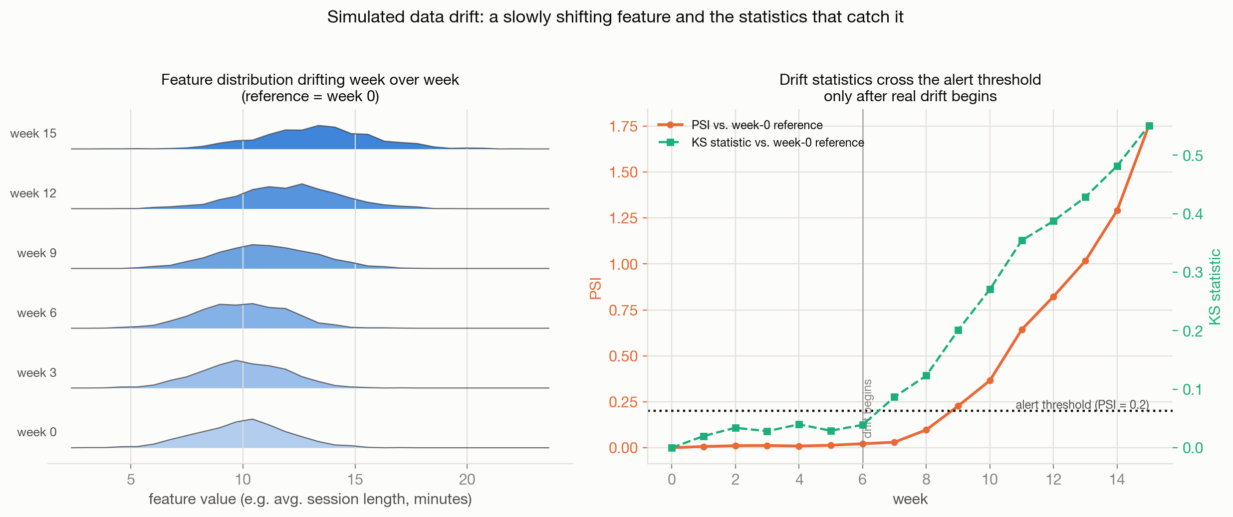
Figure 19.1 simulates exactly this: a feature’s distribution shifts its mean and variance gradually starting partway through a 16-week window, and both PSI and the KS statistic are tracked over time against the earliest week as reference. Both statistics stay flat and small while the distribution is stable, then rise and cross the conventional PSI alert threshold only after the drift has been building for a few weeks — which is itself an important operational lesson: a threshold-based drift alert always lags the onset of drift by some margin, and how large that margin is depends on how fast the drift accumulates and how sensitive the chosen statistic and threshold are.

Figure 19.1: Simulated gradual data drift and the statistics that detect it. Left: a feature’s distribution (density curves for six snapshot weeks) drifts to higher mean and wider spread starting at week 6. Right: the Population Stability Index and KS statistic, both computed against the week-0 reference distribution, stay near zero while the distribution is stable and then climb once real drift begins, crossing the conventional PSI alert threshold of 0.2 only after several weeks of accumulated shift.

Beyond drift, a short list of failure modes accounts for most production ML incidents: train/serve skew (described above); feature freshness issues, where a feature pipeline stalls or lags and the model silently serves stale inputs that look valid but aren’t current; silent dependency failures, where an upstream service degrades gracefully (returns defaults, zeros, or nulls instead of erroring) and the model treats that degraded input as real signal; latency regressions, where a model or feature computation slows down enough to violate a serving SLA, which can force fallback behavior that’s effectively an unannounced model change; miscalibration, where a model’s predicted probabilities stop reflecting true frequencies even if its ranking/discrimination is unaffected, which is especially dangerous for any downstream system that thresholds on the raw score; and logging bugs, where the pipeline that’s supposed to capture ground truth for the next round of training quietly drops, delays, or mislabels events, corrupting not today’s predictions but every future model trained on that log.

19.3 Evaluation layers

No single test catches everything, which is why production ML evaluation is usually layered by increasing cost and increasing realism, each layer catching a different class of bug:

Unit tests for feature and metric code — the cheapest layer, and the one that catches the most mundane but common bugs (a metric computed with off-by-one windowing, a feature transform that silently changes behavior on an edge case like a null or empty input).
Offline validation against held-out historical data — the standard accuracy/AUC/RMSE check, necessary but not sufficient, since it can’t catch train/serve skew, feedback loops, or anything that depends on how the model behaves once it’s actually making decisions.
Slice analysis — the same offline metrics but broken out by segment (region, device, new vs. returning user, demographic group) rather than averaged over the whole population, which is how a model that looks fine in aggregate but is quietly bad for one subgroup gets caught before launch rather than after a complaint.
Shadow tests — running the candidate model on live traffic without letting its output affect anything, purely to compare its predictions against the current production model’s, which surfaces train/serve skew and infrastructure issues (latency, crashes, resource usage) under real conditions before any user is exposed to the new model’s decisions.
A/B tests — the causal evaluation layer, covered in depth in Causal Inference and Experimentation, where the candidate model’s effect on real outcomes is measured, not just its offline predictive accuracy.
Guardrail monitoring — metrics that aren’t the primary success metric but must not regress (latency, cost, an unrelated business metric, fairness metrics across groups), watched continuously during and after rollout.
Post-launch audits — periodic, deliberate re-checks of a model that’s been live for a while, since drift and feedback loops mean a model that passed every check at launch can still degrade or develop new problems purely from operating in a changing world.

19.4 Inference optimization

Once a model is validated, serving it efficiently is its own engineering problem, with a standard toolkit:

Quantization reduces numeric precision (e.g. 32-bit floats to 8-bit integers) to shrink memory footprint and speed up inference, usually at a small, carefully measured cost in accuracy.
Distillation trains a smaller “student” model to mimic a larger “teacher,” trading some accuracy for a large reduction in serving cost and latency.
Pruning removes weights or entire structures (channels, attention heads) that contribute little to the model’s output, shrinking the model directly rather than approximating it with a smaller architecture.
Batching groups multiple inference requests together to better use parallel hardware, trading a small amount of per-request latency for much higher throughput — the central lever in serving large models cost- effectively.
Caching stores results for repeated or predictable inputs (a popular query, a frequently requested embedding) to skip inference entirely on a cache hit.
Approximate nearest neighbor (ANN) search replaces exact nearest-neighbor lookup over large embedding spaces with a sublinear approximate index, essential for any system that serves retrieval or recommendation over millions of items — see Information Retrieval, Ranking, and Recommenders.
Hardware acceleration (GPUs, TPUs, and increasingly specialized inference chips) trades cost and operational complexity for raw throughput, and is usually only worth the complexity once the other levers above have been exhausted.

19.5 When to use it / what can go wrong

When a production model’s metric regresses, the productive debugging order is almost always outside-in: check the metric definition first (did the metric itself change, or how it’s computed), then data (is the input distribution what it was — drift, a schema change, a broken upstream source), then labels (did the label definition or delay change, introducing label drift or a leakage fix that altered what “correct” means), then features (train/serve skew, a stale feature pipeline, a broken join), then the model itself (was a new version promoted, did training data or hyperparameters change), then serving (latency, a fallback path silently engaged, a routing bug sending traffic to the wrong model version), then evaluation (is the offline check that would have caught this missing, or is a slice being averaged away), and finally the product context (did user behavior itself change, a seasonal effect, a marketing campaign, a competitor’s move — sometimes the model is fine and the world changed). Working this list roughly in order, cheapest and most likely first, resolves the large majority of “the model got worse” incidents far faster than starting by re-examining the model architecture, which is usually the least likely culprit.

The broader lesson is that reliability in ML systems doesn’t come from any one component being excellent — a great model architecture doesn’t protect against a broken feature pipeline, and a great serving infrastructure doesn’t protect against silent label drift. It comes from every stage of the loop being observable (logged, monitored, alertable) and owned (someone is paged when it breaks), because the failure modes here are overwhelmingly silent by nature: nothing crashes when a feature pipeline goes stale, nothing throws an exception when training and serving compute a feature differently, and nothing pages anyone when a feedback loop slowly narrows what a recommender is willing to show. Systems that survive in production long-term are the ones built assuming these silent failures will happen, not the ones that assume the model working offline is the hard part.

19.6 How this connects

Evaluation and Benchmarking — the evaluation layers in this chapter (unit tests through post-launch audits) are the production-systems extension of the offline evaluation methodology covered there.
Causal Inference and Experimentation — A/B testing, SRM checks, and guardrail metrics are the causal layer of the evaluation stack described here, and experimentation platforms are themselves production ML systems with their own reliability requirements.
Conformal Prediction — conformal prediction sets are a natural production guardrail, flagging low-confidence or wide-interval predictions for human review or a fallback path instead of serving a bare point estimate.
Responsible, Private, and Robust AI — fairness and robustness need to be monitored in production the same way drift is, since a model that passed a fairness check at launch can develop disparate performance over time exactly like any other metric can drift.
Generative AI and Foundation Models — the inference-optimization toolkit here (quantization, distillation, batching, caching) is what makes serving large generative models economically viable, and is where most of the engineering effort in LLM infrastructure actually goes.