18 Conformal Prediction
Most models output a single number or a single softmax vector, and most consumers of that output — a dashboard, a downstream system, a human reviewer — have to decide how much to trust it with no principled way to do so. A neural network’s softmax score is not a calibrated probability; a random forest’s regression output comes with no interval at all unless you build one yourself. Conformal prediction answers a narrow but extremely useful question: instead of one number, can we wrap any trained model, of any kind, black box or not, and produce a set of plausible outputs — an interval for regression, a set of candidate labels for classification — that provably contains the true value at least \(1-\alpha\) of the time? The striking part is “provably”: the guarantee holds in finite samples, for any underlying model, however wrong or badly calibrated it is, and without assuming any parametric form for the data. That combination — distribution- free, finite-sample, model-agnostic — is not available from ordinary confidence intervals, which typically rely on asymptotic arguments or correctness of a probabilistic model. Conformal prediction gets it by relying on a much weaker and more common assumption: exchangeability.
18.1 How it works
The mechanism is built from three pieces: a nonconformity score, a calibration set, and a quantile.
A nonconformity score \(s(x, y)\) measures how “unusual” or badly a candidate label \(y\) fits input \(x\), given the trained model. For regression, the natural choice is the absolute residual, \(s(x, y) = |y - \hat f(x)|\); for classification, a common choice is one minus the model’s softmax score for that class, \(s(x, y) = 1 - \hat p(y \mid x)\). The score doesn’t need to be “correct” in any calibrated sense — it just needs to be a consistent way of ranking how surprising a label would be.
The calibration set is a batch of labeled data, held out from training and untouched by the model fit, used only to build the distribution of nonconformity scores the method needs. Compute \(s_i = s(x_i, y_i)\) for every point in the calibration set — this gives \(n\) numbers describing how nonconforming the true label was for each calibration example under the trained model.
The prediction set at level \(1 - \alpha\) for a new input \(x_{n+1}\) is then every candidate value \(y\) whose nonconformity score falls at or below the \(\lceil (n+1)(1-\alpha) \rceil / n\) empirical quantile of the calibration scores — a small finite-sample correction to the naive \((1-\alpha)\) quantile that accounts for including the test point itself in the exchangeable sequence. For regression with the absolute-residual score, this collapses to a simple symmetric interval: \(\hat f(x_{n+1}) \pm \hat q\), where \(\hat q\) is that calibration quantile. For classification, it means including every class whose \(1 - \hat p(y \mid x)\) falls below the threshold, which can produce a set with zero, one, or several labels depending on how confident the underlying model actually is on that input.
Why this gives a real guarantee. The argument is a rank argument, not an asymptotic one. If the \(n\) calibration points and the new test point are exchangeable — their joint distribution is unchanged by any permutation, which holds trivially if they’re i.i.d. but is a strictly weaker condition — then the test point’s nonconformity score is, from the model’s perspective, just one more exchangeable draw among \(n+1\) scores. Its rank among those \(n+1\) scores is uniformly distributed over \(\{1, \dots, n+1\}\), by symmetry alone: no assumption about what the scores’ distribution actually looks like is needed, only that no draw is privileged over any other. The probability that the test score falls above the chosen quantile is then exactly a counting argument over that uniform rank, which is what delivers \(P(Y_{n+1} \in C(X_{n+1})) \geq 1 - \alpha\) for any finite \(n\), for any underlying model \(\hat f\), and for any data distribution, as long as exchangeability holds. Nothing about the model needs to be well-specified; a badly fit model just produces wider, less useful intervals, but the coverage guarantee itself doesn’t depend on the model being any good.
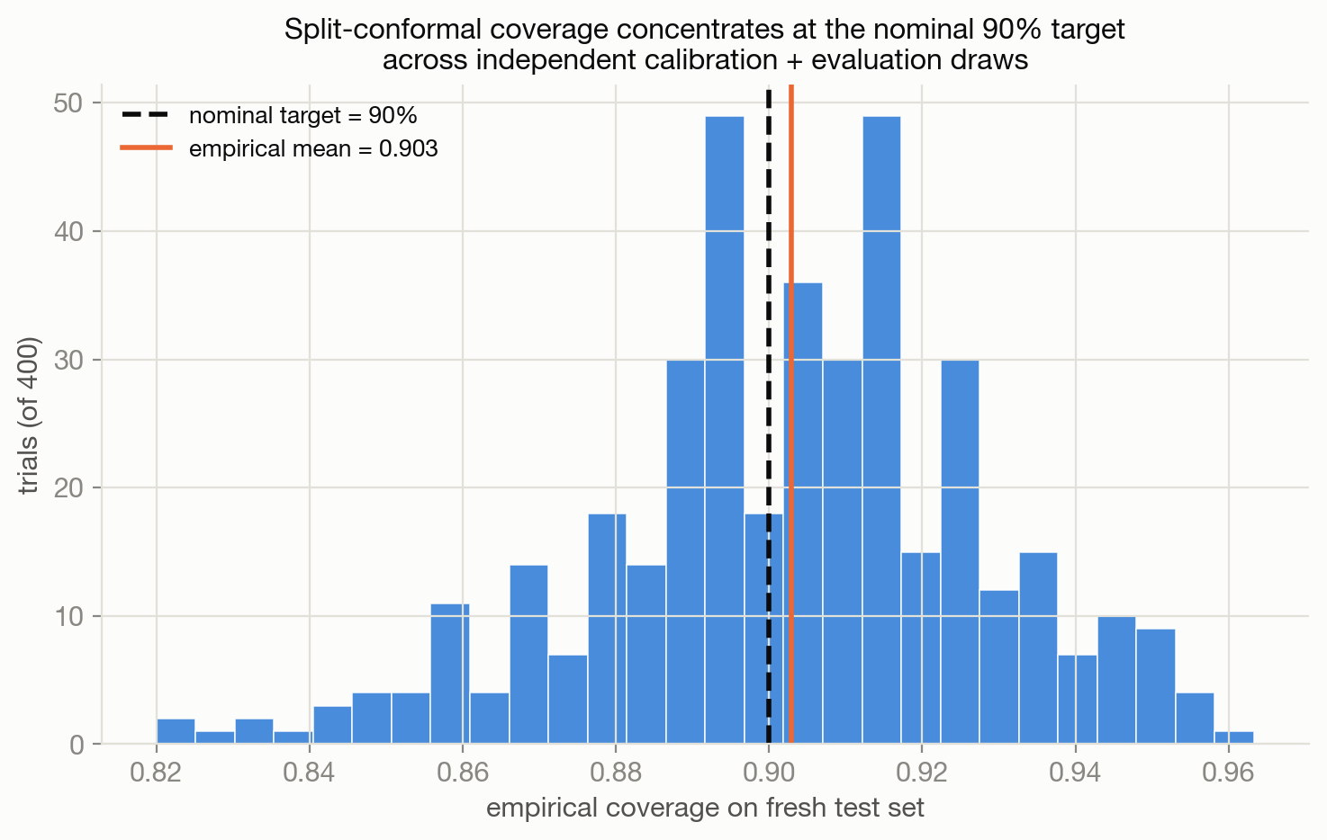
Figure 18.1 shows this empirically rather than just asserting it: a random forest is trained on synthetic heteroscedastic data, wrapped in split conformal at a 90% target, and the whole calibration-and-evaluation process is repeated 400 times on fresh random draws. The histogram of achieved coverage across those 400 independent trials concentrates tightly around 90%, exactly as the theory predicts, even though the underlying random forest is a perfectly ordinary point predictor with no notion of uncertainty built in.
Conformal prediction vs. Bayesian uncertainty
It’s worth being precise about how this relates to Bayesian uncertainty, covered in Probabilistic Modeling, because they’re often reached for in the same situations but answer different questions. A Bayesian posterior requires specifying a full probabilistic model of the data-generating process — a likelihood and a prior — and its credible intervals are only as trustworthy as that model’s assumptions; if the model is misspecified, the posterior can be confidently wrong. Conformal prediction requires no probabilistic model at all: it’s a wrapper around any point predictor, including a black-box deep network with no probabilistic interpretation, and its coverage guarantee holds in finite samples purely from exchangeability, independent of whether the underlying model is “correct” in any sense. The two are complementary rather than competing — a Bayesian posterior that is miscalibrated because of model misspecification can itself be conformalized (using, say, negative log posterior density as the nonconformity score) to restore a hard coverage guarantee on top of whatever inductive bias the Bayesian model contributes.
18.2 Main methods
- Split (inductive) conformal. The method described above: hold out one calibration set, fit the model once on the rest, compute the calibration quantile once. This is cheap — one model fit total — and is what almost every practical conformal system in production actually uses.
- Full conformal. For each candidate label \(y\) on a new input, refit the model on the training data plus the hypothetical point \((x, y)\), and check whether that refit model finds \((x,y)\) conforming. This uses data more efficiently than a fixed calibration split (no held-out set is “wasted”) and gives a tighter guarantee, but it is computationally impractical for anything beyond small models and small candidate label sets, since it means one full retrain per candidate value being tested.
- Mondrian (class-conditional) conformal. Rather than one shared calibration quantile, compute a separate quantile per group or per class. This is what you reach for when marginal (population-average) coverage isn’t good enough — for example if a classifier’s coverage would otherwise concentrate almost entirely on the majority class and starve minority classes of valid coverage. It trades a bit of statistical efficiency (fewer calibration points per group) for coverage that’s balanced across the groups that matter.
- Conformalized quantile regression (CQR). Instead of conformalizing a point predictor with a symmetric interval, first fit quantile regression models for the lower and upper bounds directly (e.g. gradient boosted quantile regressors at the \(\alpha/2\) and \(1-\alpha/2\) quantiles), then conformalize the residual between the true label and those quantile predictions. Because the base quantile regressors can already adapt interval width to each input — wider where the data is noisier, narrower where it’s easy — CQR intervals are typically much tighter than plain split conformal’s constant-width band, while keeping the same distribution-free coverage guarantee.
- Weighted / adaptive conformal. Standard conformal prediction needs exchangeability between calibration and test data, which breaks under covariate shift or non-stationary time series. Weighted conformal reweights calibration scores (often by a likelihood-ratio estimate between the calibration and test covariate distributions) to correct for a known or estimated shift; adaptive conformal inference (ACI) instead updates the target miscoverage rate online as errors are observed in a data stream, trading the strict finite-sample guarantee for a guarantee that holds asymptotically even as the underlying distribution drifts.
18.3 When to use it / what can go wrong
Conformal prediction is the tool to reach for when a system needs a hard, auditable reliability guarantee on top of an existing model — flagging low-confidence predictions for human review, bounding risk in a high-stakes decision, or providing calibrated intervals to a downstream consumer — and a full Bayesian rewrite isn’t available or isn’t worth the cost. Wrapping an existing production model conformally requires no retraining and no change to the model itself; it only needs a held-out calibration set and the light bookkeeping of computing and updating a quantile, which is why it has become the default choice for adding coverage guarantees to systems that were never built with uncertainty in mind.
Three things go wrong often enough to check for explicitly before trusting a conformal guarantee in production:
- Exchangeability isn’t automatic. The guarantee assumes the calibration set and future data are exchangeable, which typically means i.i.d. sampling from the same distribution the model will see in production. Any distribution shift between calibration and deployment — a non-stationary time series, a population that changes over time, a calibration set that was collected under different conditions than production traffic — silently breaks the guarantee, and the resulting intervals can undercover without any visible warning sign. This is exactly the failure mode addressed by weighted and adaptive conformal methods, but plain split conformal offers no protection against it on its own.
- The guarantee is marginal, not conditional. Coverage of \(1-\alpha\) holds on average over repeated draws from the calibration/test distribution — it says nothing about whether this specific interval, for this specific input, is correct. A model that’s systematically overconfident on one subgroup and underconfident on another can still hit exactly 90% marginal coverage while badly undercovering the subgroup that matters most, which is precisely the situation Mondrian conformal is built to fix by conditioning coverage on group membership rather than leaving it marginal.
- Coverage isn’t the same as usefulness. A prediction interval that spans the entire plausible range of \(y\) trivially satisfies any coverage target and is completely useless. Interval width is a separate quality axis from validity, and a badly fit underlying model — even though the conformal wrapper’s coverage guarantee holds regardless — will produce wide, uninformative sets. Improving the base model, or switching to a variant like CQR that adapts interval width per input, is how you improve usefulness without touching the validity guarantee at all.
18.4 How this connects
- Probabilistic Modeling — Bayesian posteriors and conformal prediction both quantify uncertainty but rest on different assumptions (a correct probabilistic model vs. exchangeability alone), and a Bayesian model’s miscalibration can itself be repaired by conformalizing it.
- Evaluation and Benchmarking — coverage and interval width are themselves evaluation metrics, and conformal calibration sets need the same held-out discipline as any other evaluation split to avoid leakage.
- Causal Inference and Experimentation — individual treatment effect estimates need uncertainty quantification too, and conformal methods extend to giving valid intervals around estimated effects, not just outcomes.
- ML Systems and MLOps — conformal sets are a natural production guardrail: route predictions with wide or empty conformal sets to human review or a fallback path instead of trusting a single point estimate blindly.
- Responsible, Private, and Robust AI — class-conditional (Mondrian) conformal coverage is directly a fairness tool, since it prevents a shared marginal guarantee from masking systematically worse coverage for a specific subgroup.