7 Sampling and Approximate Inference
Every probabilistic model eventually asks the same question: given this model, what do I believe? A Bayesian network gives you a posterior over hidden variables; a topic model gives you a distribution over topic assignments; a Bayesian neural network gives you a distribution over weights. In each case, “what do I believe” is a distribution, and turning it into something usable — a point estimate, a credible interval, an expected value, a decision — requires computing an integral or a sum over that distribution. That computation is called inference, and it is almost never exact.
The trouble is structural, not incidental. A joint distribution over even a modest number of discrete variables has a state space that grows exponentially, so summing over it exactly is intractable past a handful of variables. A continuous posterior might have a closed form only for a small set of convenient prior-likelihood pairs (the conjugate cases you meet in Probabilistic Modeling); step outside that set — which almost every real model does — and the normalizing constant \(p(\text{data}) = \int p(\text{data} \mid \theta)\, p(\theta) \, d\theta\) has no closed form at all. You can write the posterior down on paper; you just cannot integrate it. Sampling and approximate inference exist to answer questions about distributions you can evaluate (up to a constant) but cannot solve analytically.
7.1 How it works
The foundational trick is Monte Carlo estimation. If you want the expectation of some function \(f\) under a distribution \(p\),
\[ \mathbb{E}_p[f(x)] = \int f(x)\, p(x) \, dx, \]
and you can draw samples \(x^{(1)}, \dots, x^{(N)} \sim p\), then the sample average
\[ \hat{f}_N = \frac{1}{N} \sum_{i=1}^N f(x^{(i)}) \]
is an unbiased estimator of that expectation, and by the law of large numbers it converges to the true value as \(N \to \infty\). Crucially, the convergence rate is \(O(1/\sqrt{N})\) regardless of the dimensionality of \(x\) — unlike quadrature methods (grid-based numerical integration), which degrade exponentially with dimension. That single fact is why Monte Carlo methods dominate high-dimensional inference: the mean squared error of the estimate is governed by the variance of \(f(x)\) under \(p\), not by how many dimensions \(x\) has.
This reduces the whole inference problem to one question: how do you get samples from \(p\)? For a Gaussian or a uniform distribution, your language’s random number library already knows how. For an arbitrary unnormalized posterior \(p(\theta \mid \text{data}) \propto p(\text{data} \mid \theta)\, p(\theta)\), there is no direct sampling recipe — you cannot invert its CDF, you cannot decompose it into simpler pieces you know how to sample. The sampling and approximate-inference toolkit is a set of different answers to “how do I get samples (or a usable approximation) from a distribution I can only evaluate up to a constant.”
Two broad strategies dominate. Markov Chain Monte Carlo (MCMC) builds a Markov chain over the variable of interest whose stationary distribution is exactly the target distribution; run the chain long enough and its samples look like draws from the target, even though the chain never touches the normalizing constant. Variational inference gives up on sampling altogether and turns inference into optimization: pick a tractable family of distributions and find the member of that family closest to the true posterior. A third strategy, importance sampling, reweights samples from an easy distribution so that, in expectation, they behave like samples from the hard one. Each trades off accuracy, speed, and the kind of bias it introduces differently, which is the throughline for the rest of this chapter.
Why the Metropolis-Hastings acceptance rule is correct
It’s worth deriving this once, because the same argument underlies every MCMC method. We want to construct a Markov chain over states \(x\) whose stationary distribution is the target \(p(x)\) (known only up to a constant — write \(p(x) = \tilde{p}(x) / Z\) where \(\tilde p\) is easy to evaluate and \(Z\) is the unknown normalizer). A sufficient condition for \(p\) to be the stationary distribution is detailed balance:
\[ p(x)\, T(x \to x') = p(x')\, T(x' \to x) \]
for every pair of states \(x, x'\), where \(T\) is the chain’s transition probability. Detailed balance says the flow of probability mass from \(x\) to \(x'\) exactly equals the flow back — a stronger, easier-to-check condition than “is stationary” that implies it.
Metropolis-Hastings constructs \(T\) from two pieces: a proposal distribution \(q(x' \mid x)\) that is easy to sample from (e.g. a Gaussian centered at the current state), and an acceptance probability \(\alpha(x \to x')\) that decides whether to actually move there. The transition is \(T(x \to x') = q(x' \mid x)\, \alpha(x \to x')\) for \(x' \ne x\). Plugging into detailed balance and solving for \(\alpha\) gives the Metropolis-Hastings acceptance rule:
\[ \alpha(x \to x') = \min\left(1,\; \frac{p(x')\, q(x \mid x')}{p(x)\, q(x' \mid x)}\right) = \min\left(1,\; \frac{\tilde p(x')\, q(x \mid x')}{\tilde p(x)\, q(x' \mid x)}\right). \]
Notice the unknown normalizer \(Z\) cancels — this is the whole reason the method works on unnormalized densities. When the proposal is symmetric (\(q(x' \mid x) = q(x \mid x')\), as with a Gaussian random walk), the proposal terms cancel too and the rule reduces to the simple Metropolis ratio \(\alpha = \min(1, \tilde p(x') / \tilde p(x))\): always accept a move to a more plausible state, and accept a move to a less plausible one with probability equal to the plausibility ratio. Run this long enough and the chain’s samples are (asymptotically, after discarding an initial “burn-in” period where the chain hasn’t yet forgotten its starting point) distributed according to \(p\).
Figure 7.1 shows this in action on a target with two well-separated modes — a mixture of two Gaussians, one centered at \(-2.5\) and one at \(3.0\). The trace plot on the left shows the chain wandering within each mode for long stretches and occasionally, when a proposal happens to jump across the low-density valley and get accepted, hopping to the other mode. The histogram on the right shows that despite this stop-and-start behavior, the accumulated samples reconstruct the true bimodal density closely.
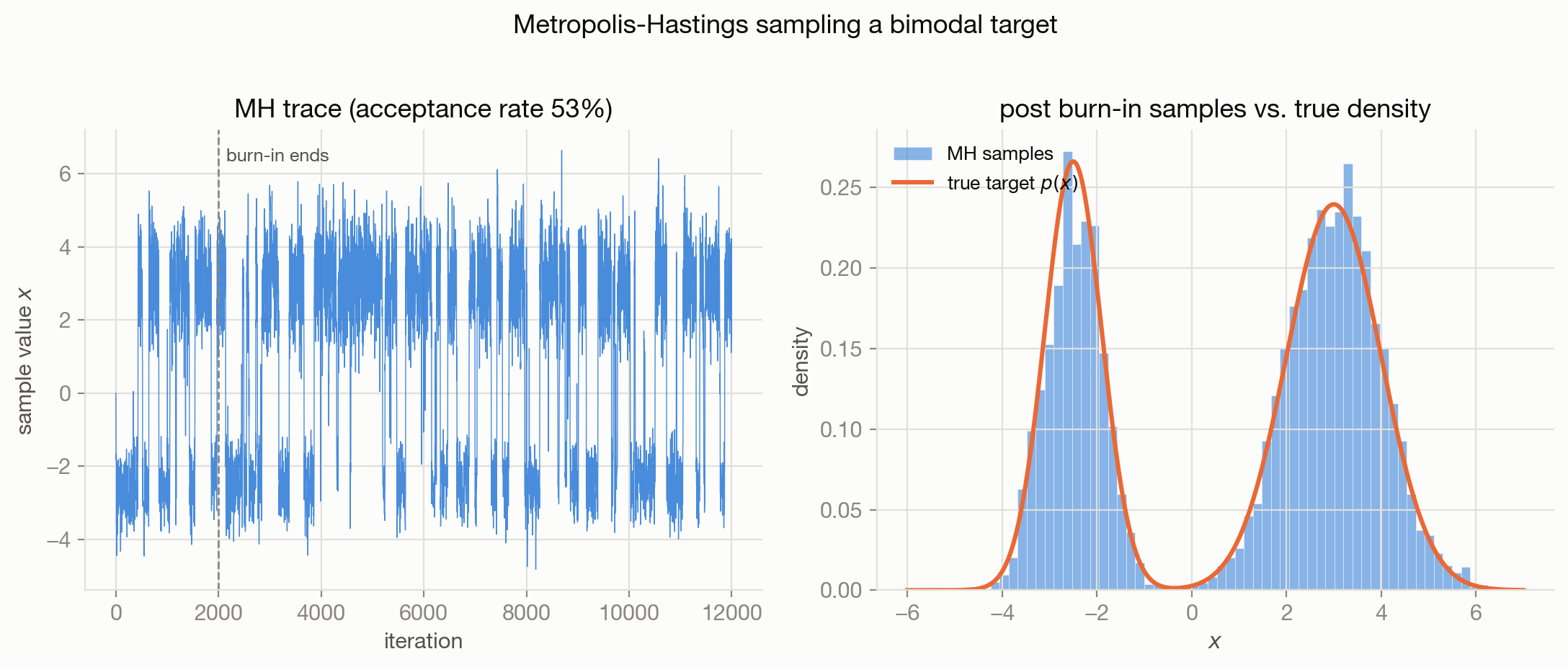
The proposal standard deviation controls a classic tradeoff visible in the trace: too small, and the chain crawls (high acceptance rate, but it takes forever to cross the low-density gap between modes — the samples are highly autocorrelated); too large, and most proposals land in low-density territory and get rejected (low acceptance rate, the chain barely moves at all). The figure uses a proposal wide enough to occasionally bridge the gap between modes, which is why the trace shows real transitions between the two levels rather than getting stuck in one.
7.2 Main methods
Metropolis-Hastings
The general-purpose MCMC method described above. Its strength is generality — it needs only a way to evaluate \(\tilde p(x)\) pointwise and a proposal distribution, so it applies to essentially any target. Its weakness is efficiency: a poorly tuned proposal (as just discussed) can make mixing extremely slow, and in high dimensions, finding a proposal scale that works well in every direction simultaneously gets hard — the acceptance rate tends to collapse as dimensionality grows unless the proposal is tuned carefully (a well-known rule of thumb targets roughly a 20-40% acceptance rate for random-walk proposals in higher dimensions).
Gibbs sampling
When the joint distribution over multiple variables is hard to sample from directly, but each variable’s conditional distribution given all the others is easy, Gibbs sampling cycles through the variables, resampling each one from \(p(x_i \mid x_{-i})\) in turn. This is a special case of Metropolis-Hastings where the proposal is the exact conditional and the acceptance probability is always 1 — every proposed move is accepted by construction, because sampling exactly from a conditional can never make the chain violate detailed balance. This makes Gibbs sampling attractive whenever a model has convenient conditional structure, which is common in graphical models (see Graphical Models and Latent Variables): Gaussian mixture assignments given cluster parameters, topic assignments given word-topic and document-topic counts in LDA, and so on. The cost is that it can mix slowly when variables are strongly correlated with each other, since each step only moves one coordinate at a time.
Hamiltonian Monte Carlo
Ordinary random-walk MCMC explores space inefficiently because a random walk covers distance proportional to \(\sqrt{N}\) in \(N\) steps — it has no memory of “which direction was good last time.” Hamiltonian Monte Carlo (HMC) fixes this by borrowing an idea from physics: it introduces an auxiliary momentum variable, treats \(-\log p(x)\) as a potential energy surface, and simulates Hamiltonian dynamics (using the gradient of \(\log p\)) to propose distant states that still land in high-probability regions, then applies a Metropolis accept/reject step to correct for numerical integration error. Because it uses gradient information, HMC can propose long, informed jumps instead of small undirected ones, dramatically reducing autocorrelation between samples in continuous, differentiable, moderate-to-high dimensional spaces. This is the mechanism behind modern probabilistic programming tools (Stan, PyMC, NumPyro), typically via its self-tuning variant, the No-U-Turn Sampler. The cost is that every step requires a gradient of the log-density and several integration sub-steps, so each iteration is more expensive than a Metropolis-Hastings step, and it doesn’t apply directly to discrete variables.
Variational inference
Variational inference (VI) reframes inference as optimization instead of simulation. Choose a family of distributions \(q_\phi(x)\) indexed by parameters \(\phi\) — often something simple like a diagonal Gaussian — and find the \(\phi\) that minimizes the KL divergence \(D_{KL}(q_\phi \| p)\) between the approximation and the true posterior. Because the true posterior is only known up to a normalizing constant, VI doesn’t minimize the KL divergence directly; instead it maximizes the evidence lower bound (ELBO),
\[ \text{ELBO}(\phi) = \mathbb{E}_{q_\phi}[\log p(\text{data}, x)] - \mathbb{E}_{q_\phi}[\log q_\phi(x)], \]
which differs from \(\log p(\text{data})\) by exactly \(D_{KL}(q_\phi \| p(x \mid \text{data})) \ge 0\) — so maximizing the ELBO is equivalent to minimizing that KL divergence, and it can be computed without ever touching the intractable normalizing constant. This is the same objective that trains variational autoencoders (see Representation Learning), where the reparameterization trick makes the ELBO differentiable with respect to \(\phi\) so it can be optimized with ordinary gradient descent. Because VI turns sampling into an optimization loop, it is typically much faster than MCMC and scales better to large datasets and high-dimensional latent spaces (it’s the default for large Bayesian neural nets and deep generative models), but it is a biased approximation: it can only represent whatever shapes the chosen family \(q_\phi\) can represent, and in practice it tends to underestimate posterior variance and can fit only one mode of a multimodal posterior (mean-field VI with independent Gaussian factors, for instance, structurally cannot represent correlation between variables or multiple separated modes).
Importance sampling
Importance sampling estimates an expectation under a hard-to-sample target \(p\) using samples drawn from an easy-to-sample proposal \(q\), reweighting each sample by the density ratio:
\[ \mathbb{E}_p[f(x)] = \int f(x) \frac{p(x)}{q(x)} q(x)\, dx \approx \frac{1}{N} \sum_{i=1}^N f(x^{(i)}) \, w(x^{(i)}), \quad x^{(i)} \sim q, \quad w(x^{(i)}) = \frac{p(x^{(i)})}{q(x^{(i)})}. \]
Unlike MCMC, the samples are independent (no chain, no mixing time, no autocorrelation) and the method is trivially parallelizable. But its variance depends entirely on how well \(q\) matches \(p\): if \(q\) puts little mass where \(p\) has a lot, a small number of samples end up with enormous weights and dominate the estimate, giving high (sometimes infinite-variance) error. This is the same mechanism behind off-policy evaluation in reinforcement learning (see Reinforcement Learning and Bandits) and behind counterfactual weighting in causal inference (see Causal Inference and Experimentation) — both reweight observations collected under one distribution to estimate quantities under another, and both inherit importance sampling’s variance blowup when the two distributions diverge.
7.3 When to use it / what can go wrong
Choosing between MCMC and VI is usually a speed-versus-fidelity call. Reach for MCMC (specifically HMC/NUTS for continuous parameters, or Gibbs when convenient conditionals are available) when you need calibrated uncertainty — a posterior whose shape you actually trust, for a low-to-moderate dimensional problem where you can afford to run thousands of iterations. Reach for VI when the model is large (deep generative models, large Bayesian neural nets, big topic models) and you need something fast enough to fit inside a training loop, and can tolerate that the posterior approximation will be biased, typically too confident.
Diagnosing MCMC convergence is not optional. A chain can look like it’s sampling productively while badly under-covering the target — this is exactly what happens if the proposal in Metropolis-Hastings never manages to bridge two modes, or if a Gibbs sampler gets stuck in one region of a strongly correlated posterior. Always run multiple chains from different starting points and check that they agree (the R-hat / Gelman-Rubin diagnostic formalizes this); look at trace plots for a well-mixed chain that looks like noise around a stable mean, not slow drift or long flat stretches; and discard an adequate burn-in period. A single short chain that “looks fine” is the most common way sampling-based inference silently gives wrong answers.
Watch for high-variance importance weights. If effective sample size (a standard diagnostic, roughly \(1 / \sum_i w_i^2\) for normalized weights) is much smaller than the nominal number of samples, your importance-sampling estimate is effectively being driven by a handful of samples and should not be trusted, no matter how large \(N\) nominally is.
Mind the cost of gradient-based samplers. HMC needs the gradient of the log-density at every leapfrog sub-step, which means it needs a differentiable model — fine for a continuous Bayesian regression or a neural network’s weights, not directly applicable to models with discrete latent variables (mixed discrete-continuous models typically combine HMC for the continuous part with Gibbs steps for the discrete part).
Approximate inference does not mean “roughly correct answer, don’t worry.” Reported credible intervals and posterior means are only as good as the sampler’s coverage or the variational family’s expressiveness. In production systems that make decisions off posterior uncertainty (active learning, Bayesian optimization, risk-aware ranking), an under-covering approximation silently produces overconfident decisions — this is one reason Conformal Prediction exists as a model-agnostic alternative that gives distribution-free coverage guarantees without relying on the sampler or variational family being correct.
7.4 How this connects
- Probabilistic Modeling sets up exactly the objects — likelihoods, priors, posteriors, evidence — that sampling and VI exist to compute; this chapter is the “how do you actually get the numbers” companion to that chapter’s “what do the numbers mean.”
- Graphical Models and Latent Variables supplies the conditional-independence structure that makes Gibbs sampling and the E-step of EM tractable — Gibbs sampling is, in effect, a stochastic relative of EM that samples hidden variables instead of taking their expectation.
- Representation Learning uses the ELBO and the reparameterization trick directly: a variational autoencoder is variational inference where the approximate posterior is produced by a neural encoder and optimized with the same machinery introduced here.
- Generative AI and Foundation Models depends on sampling at inference time in a different sense — autoregressive decoding and diffusion’s iterative denoising are both sequential sampling procedures, and diffusion models in particular can be read as running a learned Markov chain toward a data distribution, echoing the MCMC ideas here.
- Reinforcement Learning and Bandits reuses importance sampling directly for off-policy evaluation — estimating the value of one policy using data collected under another — and inherits the same variance-blowup failure mode discussed above.