10  Sequence, Time-Series, and State Models

Most of the models covered so far treat each example as independent: a row of features, a label, done. A huge amount of real data is not like that — order carries meaning. A sentence’s words mean something different in a different order; a patient’s vital signs today are only interpretable relative to yesterday’s; a stock price is a trajectory, not a point. Sequence and state models are the family of tools built for exactly this case: data where position, order, and time carry information the model has to use, and where what happens next plausibly depends on some evolving internal condition — a “state” — that isn’t always directly observed.

The unifying idea across this whole chapter is that an evolving process can be modeled either by tracking an explicit state and specifying how it moves (Markov chains, hidden Markov models, state-space models) or by letting a neural network learn an implicit notion of state and its dynamics directly from data (RNNs, LSTMs, transformers). Both approaches answer the same underlying question — what do I need to remember about the past to predict the future — but they differ enormously in how much structure they assume versus how much they leave for the model to discover, which is the main axis this chapter uses to compare them.

10.1 How it works

The Markov assumption

The simplest possible sequence model is a Markov chain: a sequence of states \(s_1, s_2, \dots, s_T\) where the probability of the next state depends only on the current state, not on the full history:

\[ p(s_{t+1} \mid s_1, \dots, s_t) = p(s_{t+1} \mid s_t). \]

This is a strong, often false, but enormously useful simplifying assumption. It compresses what would otherwise be an intractable dependence on arbitrarily long history into a single transition distribution \(p(s_{t+1} \mid s_t)\), representable as a simple transition matrix for discrete states. Almost every other model in this chapter is best understood as a way of relaxing or working around this assumption: hidden Markov models keep the Markov assumption but on a state you don’t directly observe; RNNs keep the “compress history into a fixed-size summary” spirit but let a neural network learn what to summarize instead of assuming first-order Markov structure; transformers abandon the compression assumption almost entirely and let the model look at the full history directly through attention.

Hidden Markov models and why Viterbi is exact dynamic programming

A hidden Markov model (HMM) assumes there’s a hidden state sequence \(z_1, \dots, z_T\) evolving with Markov dynamics, \(p(z_{t+1} \mid z_t)\), and that each hidden state emits an observation \(x_t\) with probability \(p(x_t \mid z_t)\) — but you only ever see the observations, never the hidden states directly. This is the right model whenever you believe some noisy, observed signal is being driven by an underlying condition that changes more slowly or more structurally than the noise itself: a sensor reading driven by an unobserved machine health state, a sequence of words driven by unobserved part-of-speech tags, market returns driven by an unobserved volatility regime.

Given an observed sequence and a known (or fitted) HMM, the natural question is: what’s the most likely hidden state sequence that produced it? Brute force is hopeless — for \(T\) time steps and \(K\) hidden states there are \(K^T\) possible sequences. The Viterbi algorithm solves this exactly, in \(O(T K^2)\) time, using dynamic programming. The key insight is that the best path ending at state \(k\) at time \(t\) only needs to know the best score of paths ending at each state at time \(t-1\) — you never need to reconsider earlier time steps once you’ve recorded the best score into each state at the current step. Define

\[ \delta_t(k) = \max_{z_1, \dots, z_{t-1}} p(z_1, \dots, z_{t-1}, z_t = k, x_1, \dots, x_t), \]

the probability of the single best path ending in state \(k\) at time \(t\) having generated the observations seen so far. This satisfies a clean recursion:

\[ \delta_t(k) = \left[\max_j \; \delta_{t-1}(j) \, p(z_t = k \mid z_{t-1} = j)\right] \cdot p(x_t \mid z_t = k), \]

built up left to right across the sequence while also recording, at each step, which previous state \(j\) achieved the max (the backpointer \(\psi_t(k)\)). Once you reach \(t = T\), the state with the highest \(\delta_T\) gives the end of the optimal path, and following the backpointers from there back to \(t=1\) recovers the entire most-likely hidden state sequence — one forward pass to compute scores, one backward pass to read off the path, both linear in sequence length. In practice this recursion is computed in log-space (summing log-probabilities instead of multiplying probabilities) purely for numerical stability, since a raw product of many probabilities underflows to zero quickly.

Figure 10.1 shows Viterbi decoding on a small hand-specified HMM with two hidden states (“calm” and “volatile,” meant to evoke a volatility regime) and three possible emission symbols (“small,” “medium,” “large” moves). A true hidden path is simulated from the model’s own transition matrix, noisy observations are simulated from the emission matrix, and Viterbi is run on the observations alone — without ever seeing the true hidden path — to recover its best guess. The decoded path tracks the true path closely but not perfectly: the highlighted mismatches are exactly where the emitted symbol was ambiguous enough (a “small” move emitted during a volatile period, or a “medium” move emitted during a calm one) that the most probable explanation, given only the transition and emission probabilities, differs from what actually generated it. This is the honest picture of what Viterbi gives you: the single best explanation consistent with the model and the observed evidence, not a guarantee of recovering the literal truth.

Figure 10.1: A small two-state HMM (“calm” vs. “volatile”) decoded with the Viterbi algorithm. Top: the true hidden state path used to simulate the data. Middle: the Viterbi-decoded path recovered from the noisy observations alone, with shaded bands marking the handful of time steps where it disagrees with the truth — these occur exactly where the emitted symbol was ambiguous between the two states. Bottom: the noisy observed emissions that are all Viterbi actually has access to.

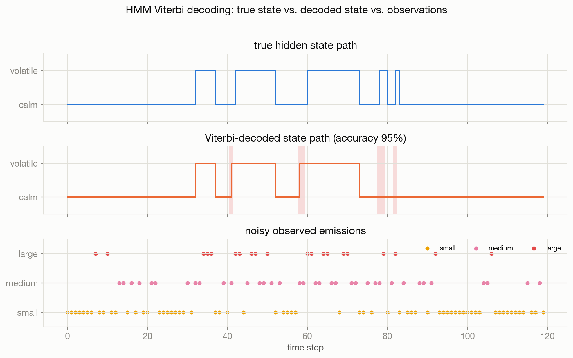
State-space models

State-space models generalize the HMM picture from discrete hidden states to continuous ones, and from arbitrary transition/emission distributions to (in the classic case) linear-Gaussian dynamics: a continuous hidden state \(z_t\) evolves as \(z_t = A z_{t-1} + \text{noise}\), and is observed through \(x_t = C z_t + \text{noise}\). The Kalman filter is the exact, closed-form recursive solution for inferring \(z_t\) in this linear-Gaussian case — it’s the continuous-state, closed-form analogue of what Viterbi does for discrete-state HMMs, propagating a Gaussian belief over the hidden state forward in time and updating it with each new observation using exact Bayesian updates (no sampling or approximation needed, because Gaussian priors and linear-Gaussian likelihoods stay Gaussian under Bayes’ rule). When the dynamics or observation model are nonlinear, exact inference is lost and you fall back to approximations (the extended or unscented Kalman filter) or the general-purpose sampling and variational tools from Sampling and Approximate Inference.

10.2 Main methods

Neural sequence models

• RNNs process a sequence one step at a time, maintaining a hidden state \(h_t = f(h_{t-1}, x_t)\) that is meant to summarize everything relevant about the sequence so far. In principle this gives an RNN unbounded context; in practice, backpropagation through time multiplies gradients across every time step the same way backpropagation through depth multiplies gradients across layers (see Deep Learning Foundations), so vanilla RNNs suffer badly from vanishing (and occasionally exploding) gradients over long sequences, making them unable to reliably learn long-range dependencies.
• LSTMs (and the closely related GRUs) fix this with a gating mechanism: a separate cell state that information can flow through nearly unchanged across time steps, modulated by learned gates that decide what to keep, what to overwrite, and what to output at each step. This is the same “give the gradient an unimpeded path” idea as a residual connection, applied across time instead of across depth, and it’s why LSTMs could learn dependencies spanning hundreds of steps where vanilla RNNs typically couldn’t.
• Transformers replace recurrence with self-attention (derived in Deep Learning Foundations), letting every position attend directly to every other position rather than relying on information being carried forward step by step through a hidden state. This removes the vanishing-gradient-over-time problem almost entirely (there’s no long chain of sequential multiplications between distant time steps) and allows full parallelism across the sequence during training, at the cost of attention’s quadratic compute and memory cost in sequence length, and the need for an explicit positional signal (since attention itself has no inherent notion of order) — usually positional encodings or embeddings added to each token.
• Temporal convolution models apply causal, dilated convolutions along the time axis — “causal” meaning each output only depends on past inputs, never future ones, which matters for anything used autoregressively or online. They sit between RNNs and transformers on several axes: more parallelizable than an RNN (convolutions over different positions can be computed simultaneously), and with a receptive field that grows only linearly (or with dilation, geometrically) in the number of layers rather than covering the whole sequence in one layer the way attention does, which caps their compute cost more predictably than full self-attention on very long sequences.

Time-series specific structure

Time series carry extra structure beyond generic sequence modeling that’s worth naming directly: trend (a slow, systematic drift in the level of the series over time), seasonality (a repeating pattern at a known, fixed period — daily, weekly, yearly), and autocorrelation (the correlation of the series with lagged versions of itself, which is what makes a time series a time series rather than i.i.d. noise, and what classical models like ARIMA are built to capture directly). Forecasting adds practical concerns that don’t arise in generic sequence prediction: the forecasting horizon (how far ahead you’re predicting strongly affects both achievable accuracy and appropriate model complexity — a one-step-ahead forecast and a one-year-ahead forecast are different problems even on the same series), exogenous variables (external signals, like weather or promotions, that help explain the series but aren’t generated by the same process being forecast), backtesting (evaluating a forecasting model by rolling it forward through historical time and checking predictions against what actually happened next, always respecting time order — never letting a model see future data during evaluation, which is a specific, easy-to-miss form of the data leakage discussed in Deep Learning Foundations), and forecast residual anomaly detection (once you have a forecasting model, unusually large forecast errors are themselves a signal — a spike in the residual between predicted and actual values often flags an anomaly more sensitively than watching the raw series, because it accounts for expected trend and seasonality first).

10.3 When to use it / what can go wrong

Match model complexity to what you actually need to explain. A Markov chain is the right tool when the process genuinely has short memory and you need something simple, fast, and interpretable (next-page prediction, basic churn modeling). An HMM is right when you believe there’s a meaningfully different, unobserved regime driving the observations and you want that regime made explicit and inspectable — the discreteness and interpretability of “which hidden state is active” is often the whole point, not a limitation. A Kalman filter or general state-space model is right for continuous physical or quasi-physical dynamics (tracking, sensor fusion) where linear-Gaussian assumptions are reasonable and you want fast, exact, principled uncertainty propagation. Reach for LSTMs or transformers only once you need to model dependencies too complex or too long-range for these structured alternatives, or when you have enough data that a highly flexible model won’t just overfit noise — the extra flexibility of a neural sequence model is not free, and on a short, simple, low-data series a well-specified statistical model will often beat it.

Sequence length and serving constraints should shape the architecture choice as much as accuracy does. Attention’s quadratic cost in sequence length becomes the binding constraint on very long sequences (long documents, long user histories, high-frequency sensor streams) well before accuracy differences between architectures do; this is a large part of why production sequence models on very long inputs still lean on recurrent state, windowed/sparse attention, or hybrid architectures rather than full dense attention, and it’s a direct instance of the systems-cost thinking covered in ML Systems and MLOps.

Backtesting mistakes are the most common way a time-series model looks good offline and fails in production. Any preprocessing step — scaling, imputation, feature construction — fit on the whole dataset before a train/test split leaks future information into the past; any evaluation window that isn’t strictly forward in time (shuffling time series data the way you would i.i.d. tabular data) silently inflates offline accuracy. Always backtest by rolling forward in time, retraining or updating only on data available at each point being evaluated.

Regime change breaks every one of these models the same way distribution shift breaks any statistical model — a transition matrix, an HMM’s emission distribution, or a neural sequence model’s learned dynamics are all fit to historical behavior, and none of them automatically detect that the underlying process has changed. Forecast residual monitoring (mentioned above) is one of the more reliable early-warning signals for this, precisely because it’s watching for the model’s own predictions to start being systematically wrong.

Interpretability tends to trade off against flexibility here just as sharply as in the rest of deep learning. An HMM’s hidden states and transition probabilities can be inspected directly; a transformer’s internal “state” (its full attention pattern and residual stream across layers) is much harder to summarize into something a human can reason about. When a stakeholder needs to understand why a sequence model made a particular prediction — a regulator, a clinician, an operator debugging an anomaly — that need should inform the choice of model, not just be handled after the fact with post-hoc explanation tools.

10.4 How this connects

• Graphical Models and Latent Variables is where the HMM belongs formally — it’s a specific instance of a latent-variable graphical model with a chain-structured dependency graph, and the EM algorithm covered there is exactly what’s used to fit an HMM’s transition and emission parameters when they aren’t known in advance (Viterbi assumes they are; the Baum-Welch algorithm, a specialization of EM, learns them from data).
• Sampling and Approximate Inference is the fallback once a state-space model’s dynamics stop being linear-Gaussian and exact Kalman-filter inference is no longer available — particle filters (a sequential Monte Carlo method) and MCMC extensions handle nonlinear, non-Gaussian state-space inference using the same sampling principles introduced there.
• Deep Learning Foundations supplies the backpropagation-through-time mechanics, the vanishing-gradient problem, and the attention mechanism that this chapter’s neural sequence models are built directly on top of.
• Causal Inference and Experimentation intersects with time-series forecasting whenever the question shifts from “what will happen” to “what would have happened under a different intervention” — forecasting a counterfactual trend is a common building block in causal impact analysis for time-ordered data.
• Generative AI and Foundation Models builds directly on the transformer and autoregressive sequence machinery here — a large language model is, at the mechanical level, an autoregressive sequence model over tokens, trained and decoded with the same next-step conditioning logic as any other sequence model in this chapter, just at a very different scale.