5 Probabilistic Modeling
A supervised model that outputs “0.73” is making a claim, but a plain point prediction leaves that claim ambiguous — is 0.73 a probability the model is fairly confident in, or a wild guess that happens to land there? Probabilistic modeling is the discipline of making that claim explicit: instead of producing a single best guess, you write down a full probability distribution over the quantity you don’t know — a label, a hidden cluster assignment, a parameter, a future observation — and reason about it using the rules of probability rather than a point estimate and a loss function alone. This matters whenever uncertainty itself is part of the answer: when data is scarce and you want your model to say “I don’t know” rather than confidently guess, when labels are noisy and you want to model that noise rather than pretend it isn’t there, when there’s real prior knowledge worth encoding before seeing any data, or when a downstream decision needs a calibrated probability rather than a ranking. It is also, as the previous two chapters kept gesturing toward, the framework that most of supervised learning turns out to be a special case of.
5.1 How it works
The vocabulary, made precise
A few terms get thrown around loosely enough that it’s worth pinning down exactly what each one means, because the entire framework is just these pieces assembled in a specific order. A random variable is a quantity whose value is uncertain — a coin’s next flip, a user’s true preference, a model’s weight. A distribution assigns probability (or probability density, for continuous variables) to each possible value. The likelihood \(p(\text{data} \mid \theta)\) is a distribution over data, but evaluated at the data you actually observed and viewed as a function of the unknown parameter \(\theta\) — it answers “how probable is the data I saw, for each candidate value of \(\theta\)?” The prior \(p(\theta)\) encodes what you believed about \(\theta\) before seeing any data. The posterior \(p(\theta \mid \text{data})\) is the updated belief after seeing data — this is usually the thing you actually want. The evidence \(p(\text{data})\) is a normalizing constant, the total probability of the observed data marginalized over every possible \(\theta\); it’s what makes the posterior integrate to 1, and it’s also, not coincidentally, the hardest of these five quantities to compute in general (the entire next chapter, on sampling and approximate inference, exists largely to work around this difficulty).
The core conceptual distinction that trips people up first is likelihood versus posterior, because they involve the exact same joint quantity \(p(\text{data}, \theta)\) read in two different directions. The likelihood fixes the data (it happened, it’s given) and asks how probable that data would have been under each candidate parameter value — it is a function of \(\theta\), not a probability distribution over \(\theta\), and it need not integrate to 1 over \(\theta\). The posterior fixes nothing and asks, given that we now know the data, how plausible each value of \(\theta\) is — it is a proper probability distribution over \(\theta\). Confusing the two is a common and consequential error: “the likelihood of \(\theta=0.7\) is high” means the observed data would have been probable if \(\theta\) were 0.7; it does not by itself mean \(\theta=0.7\) is probable, which additionally depends on the prior.
Bayes’ rule
The mechanism that turns a likelihood and a prior into a posterior is Bayes’ rule, which falls directly out of the definition of conditional probability applied twice:
\[ p(\theta \mid x) = \frac{p(x \mid \theta)\, p(\theta)}{p(x)} = \frac{p(x \mid \theta)\, p(\theta)}{\int p(x \mid \theta')\, p(\theta')\, d\theta'} \]
In words: posterior is proportional to likelihood times prior, renormalized by the evidence so the result is a valid distribution. The proportionality form — \(p(\theta \mid x) \propto p(x \mid \theta)\, p(\theta)\) — is usually the more useful one to keep in your head, because it says the shape of the posterior over \(\theta\) is entirely determined by likelihood times prior; the evidence only rescales it to integrate to 1, and for many purposes (finding the mode, comparing relative plausibility of two parameter values, MCMC sampling) you never need to compute it explicitly at all.
A worked update: Beta-Binomial
The cleanest way to see this mechanism operate is a case where every piece has a closed form. Suppose you’re estimating the bias \(\theta\) of a coin — equivalently, a conversion rate, a click-through rate, any binary success probability. You start with a prior belief \(\theta \sim \mathrm{Beta}(a_0, b_0)\), whose density is proportional to \(\theta^{a_0-1}(1-\theta)^{b_0-1}\); \(\mathrm{Beta}(1,1)\) is the uniform distribution on \([0,1]\), representing genuine ignorance about \(\theta\) before seeing anything. Now you observe \(n\) independent coin flips with \(k\) heads. The likelihood of that data given \(\theta\) is Binomial: \(p(k \mid \theta, n) \propto \theta^k (1-\theta)^{n-k}\). Multiplying likelihood by prior:
\[ p(\theta \mid k, n) \propto \theta^k(1-\theta)^{n-k} \cdot \theta^{a_0-1}(1-\theta)^{b_0-1} = \theta^{a_0+k-1}(1-\theta)^{b_0+n-k-1} \]
which is — by inspection of the exponents — exactly the shape of a \(\mathrm{Beta}(a_0 + k,\, b_0 + n - k)\) distribution. The posterior is again a Beta distribution, just with its parameters shifted by the observed counts: \(a\) increases by the number of successes, \(b\) by the number of failures. This is what makes the Beta prior conjugate to the Binomial likelihood — the posterior has the same functional family as the prior, so updating is pure arithmetic on the parameters, no integration required, and the posterior from one batch of data becomes the exact prior for the next batch, which is what makes this the natural mechanism for online, streaming belief updates (A/B test monitoring, bandit algorithms).
Figure 5.1 runs this update on a simulated sequence of coin flips with a true bias of 0.7, starting from a flat \(\mathrm{Beta}(1,1)\) prior.
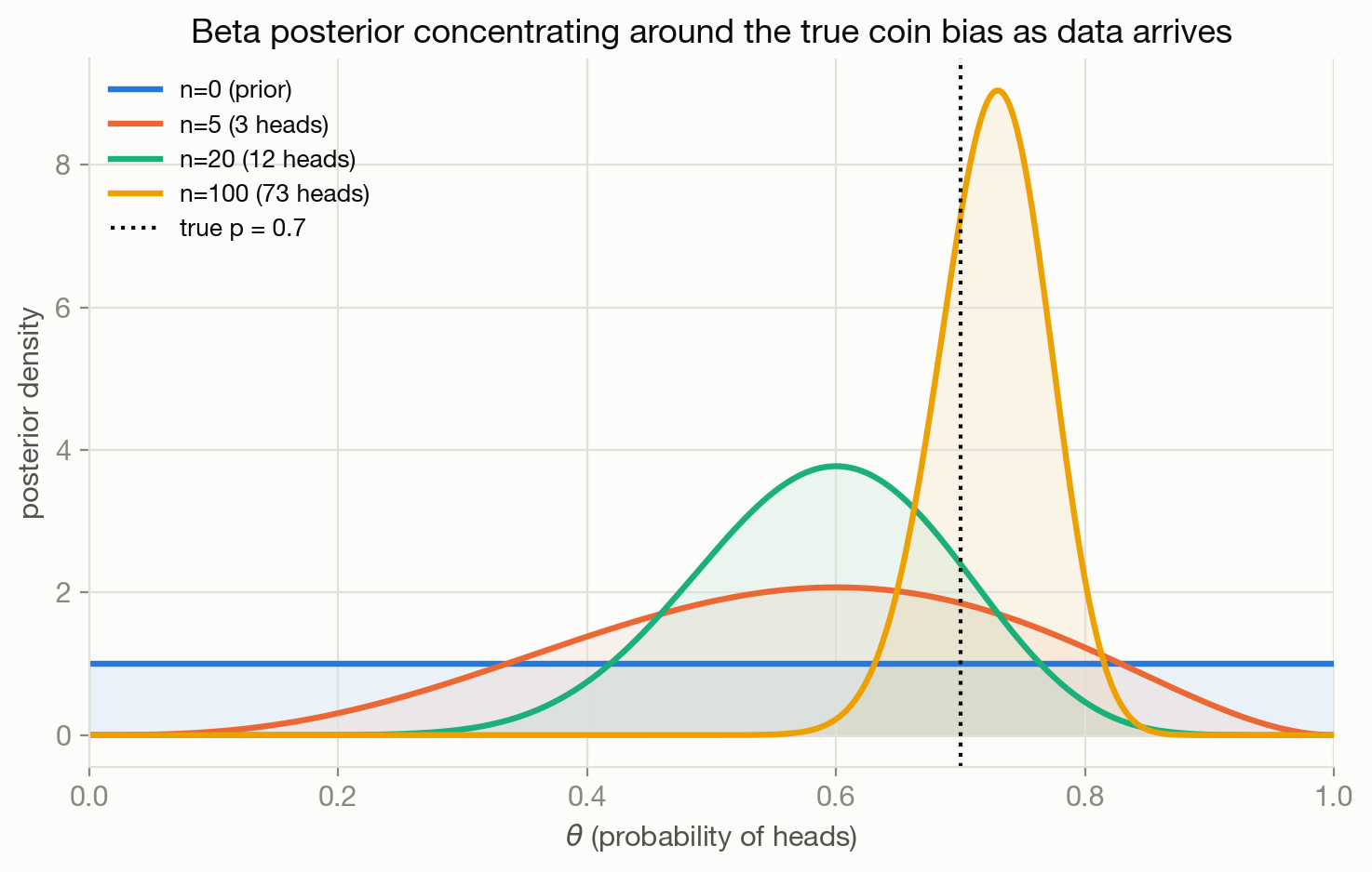
Two things are worth noticing in that figure beyond the obvious concentration around the true value. First, with only 5 flips the posterior is still very wide — barely different in spread from the prior — which is the correct behavior: 5 coin flips genuinely don’t tell you much, and a probabilistic model says so explicitly, whereas a bare point estimate (3/5 = 0.6) would report a number with no indication of how little it should be trusted. Second, the posterior mean with a \(\mathrm{Beta}(1,1)\) prior after \(n\) flips and \(k\) heads is \((k+1)/(n+2)\) — the prior acts like two “pseudo-observations” (one implicit success, one implicit failure) that get diluted as real data accumulates, exactly the shrinkage-toward-a-default behavior that regularization provides in the ERM framework of the previous chapters. This is not a coincidence; it’s the same mechanism, viewed from the Bayesian side.
Generative versus discriminative models
A model is generative if it specifies how the full data — inputs and labels together — are assumed to have been produced: it models \(p(x, y)\), or equivalently \(p(x \mid y)\,p(y)\), describing a story of how you’d sample a label and then sample features conditioned on that label. A model is discriminative if it models only \(p(y \mid x)\) directly, the conditional distribution of the label given the features, without any commitment to how \(x\) itself arose. Naive Bayes is the canonical generative classifier: it assumes a class prior \(p(y)\) and a (conditionally independent, given the class) feature likelihood \(p(x \mid y)\), then uses Bayes’ rule to flip that around into \(p(y \mid x)\) at prediction time. Logistic regression is the matched discriminative counterpart: it models \(p(y\mid x)\) directly via the sigmoid of a linear function, with no model of \(p(x)\) at all.
The practical tradeoff is real and goes both ways. A generative model can be trained with unlabeled data folded into estimating \(p(x)\), can handle missing features naturally by marginalizing them out, and can generate synthetic samples — properties a discriminative model doesn’t have because it never modeled \(p(x)\) to begin with. But those properties come at a cost: getting \(p(x \mid y)\)’s shape wrong (e.g. naive Bayes’ feature-independence assumption, which is almost always literally false) can hurt classification accuracy, whereas a discriminative model, by only ever committing to the decision boundary and not to how the data was generated, is often more accurate for classification specifically, precisely because it isn’t spending modeling effort on a part of the problem (the marginal \(p(x)\)) that pure classification doesn’t need. Naive Bayes and logistic regression converge to the same decision boundary under certain distributional assumptions, but they get there by fitting very differently shaped objectives, and which one wins in practice depends heavily on the sample size and how badly the generative assumptions are violated.
5.2 Main methods
Bernoulli, categorical, Gaussian, Poisson. The basic building-block distributions, each matched to a different kind of data: Bernoulli for a single binary outcome, categorical for one-of-\(K\) outcomes, Gaussian for continuous real-valued measurements, Poisson for non-negative integer counts. Almost every probabilistic model in this chapter and the next is built by composing these primitives — picking the right one for your data’s actual support (not defaulting to Gaussian because it’s familiar) is itself a meaningful modeling decision.
Naive Bayes. A generative classifier that assumes features are conditionally independent given the class label — a strong, usually false assumption, but one that makes both fitting (just count/average within each class) and inference trivially fast, and that turns out to work surprisingly well for high-dimensional, sparse data like text, where the independence assumption’s damage is limited relative to the benefit of having a simple, low-variance estimator with very little data per parameter.
Gaussian mixture models. A generative model for clustering: assume each data point was generated by first picking one of \(K\) hidden clusters according to some mixing proportions, then drawing from that cluster’s own Gaussian distribution. Unlike k-means, which assigns each point to exactly one cluster and assumes clusters are spherical and equally sized, a GMM produces soft, probabilistic cluster assignments and can fit clusters of different shapes, sizes, and orientations via each cluster’s own covariance matrix. Fitting one requires an iterative algorithm (EM) rather than a closed form, which is the subject of the next chapter.
Bayesian linear regression. Ordinary linear regression with an explicit prior over the coefficients, producing a full posterior distribution over \(\beta\) instead of a single point estimate — which is exactly the ridge regression connection from the supervised learning chapter made fully probabilistic: the MAP estimate under a Gaussian prior is ridge regression, but the Bayesian version additionally gives you the posterior’s spread, which translates directly into calibrated predictive uncertainty (wider intervals where you have less data or are extrapolating) rather than just a shrunk point estimate.
Probabilistic matrix factorization. Models a user-item ratings matrix as generated from low-dimensional latent user and item vectors plus noise: \(r_{ui} \sim \mathcal{N}(u_u^\top v_i, \sigma^2)\). This is the probabilistic lens on the matrix factorization used throughout recommender systems — it turns a plain least-squares factorization into a model that naturally handles missing entries (most of the matrix, in practice), supports regularization as priors on \(u\) and \(v\), and can produce uncertainty estimates on predicted ratings for cold or sparse users/items.
Topic models. Generative models for documents-as-mixtures-of-topics (most prominently Latent Dirichlet Allocation): each document is assumed to be generated by drawing a distribution over topics, then for each word, drawing a topic from that distribution and a word from that topic’s word distribution. Recovering the topics and per-document mixtures from only the observed words is a latent-variable inference problem of the same family covered in the next chapter, and topic models were the dominant approach to unsupervised text structure before learned embeddings and language models displaced them for most practical use.
5.3 When to use it / what can go wrong
Reach for explicit probabilistic modeling when the problem has one or more of: genuinely noisy or partially unreliable labels you want to model rather than treat as ground truth, missing data you need to handle principledly rather than by imputing and hoping, real prior domain knowledge worth encoding (a known plausible range for a parameter, a known base rate), meaningfully small data where a point estimate would be overconfident, or a downstream decision that needs a calibrated probability or a full predictive distribution rather than a ranking or a single guess.
Model misspecification is silent. Every probabilistic model encodes assumptions — Gaussian noise, conditional independence, a particular link function — and if those assumptions are badly wrong, the posterior can be confidently wrong rather than appropriately uncertain; Bayesian updating makes you more certain as more (misspecified-model) data arrives, not less, which is the opposite of what you’d want if the model itself is the problem. Posterior predictive checks — simulating data from the fitted model and comparing it to the real data — are the standard defense, and should be routine, not optional.
Prior sensitivity with small data. With few observations, the posterior can be dominated by the prior rather than the data, which is sometimes exactly the desired behavior (regularization) and sometimes a sign you’re smuggling in an assumption that deserves scrutiny — always check how much the posterior actually shifts when you change the prior to something else reasonable, especially before reporting a Bayesian result as if it were purely data-driven.
Computational cost of exact inference. The evidence term \(p(x)\) in Bayes’ rule requires integrating over every possible parameter value, which has a closed form only for conjugate prior/likelihood pairs like the Beta-Binomial example above. Anything more realistic — nonconjugate priors, hierarchical models, latent variables interacting nonlinearly — typically has no closed- form posterior, which is exactly the problem the sampling and variational inference methods in Sampling and Approximate Inference exist to solve.
Conflating likelihood with posterior, or point estimates with full distributions. As discussed above, reporting “the likelihood favors \(\theta=0.7\)” as if it meant “\(\theta\) is probably 0.7” ignores the prior entirely; reporting a posterior mean without its spread throws away most of the reason to have gone Bayesian in the first place. If uncertainty quantification was the point of the exercise, the final artifact needs to be a distribution or an interval, not a single number.
5.4 How this connects
- Supervised Learning is where this chapter’s machinery was already operating in disguise: cross-entropy loss is Bernoulli/categorical negative log-likelihood, and \(\ell_2\)/\(\ell_1\) regularization are Gaussian/Laplace priors under MAP estimation — this chapter just makes that framing explicit and complete.
- Graphical Models and Latent Variable Models extends everything here to structured collections of random variables and to models with hidden variables that must themselves be inferred, using the EM algorithm to fit exactly the GMM sketched above.
- Sampling and Approximate Inference is the direct answer to the “computational cost of exact inference” limitation flagged above — MCMC and variational inference are how you get a usable posterior when conjugacy doesn’t hand you one for free.
- Conformal Prediction offers a distribution-free alternative route to calibrated uncertainty that doesn’t require committing to a full generative probability model at all, useful precisely when the model-misspecification risk above is a serious concern.
- Causal Inference and Experimentation shares this chapter’s generative instinct — modeling how data was actually produced — but pushes it further, toward asking what data would have been produced under an intervention that didn’t happen, which plain probabilistic modeling of observed data alone cannot answer.